The tutorial provides a number of "Excel if contains" formula examples that show how to return something in another column if a target cell contains a required value, how to search with partial match and test multiple criteria with OR as well as AND logic.
One of the most common tasks in Excel is checking whether a cell contains a value of interest. What kind of value can that be? Just any text or number, specific text, or any value at all (not empty cell).
There exist several variations of "If cell contains" formula in Excel, depending on exactly what values you want to find. Generally, you will use the IF function to do a logical test, and return one value when the condition is met (cell contains) and/or another value when the condition is not met (cell does not contain). The below examples cover the most frequent scenarios.
If cell contains any value, then
For starters, let's see how to find cells that contain anything at all: any text, number, or date. For this, we are going to use a simple IF formula that checks for non-blank cells.
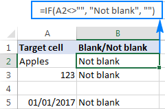
For example, to return "Not blank" in column B if column A's cell in the same row contains any value, you enter the following formula in B2, and then double click the small green square in the lower-right corner to copy the formula down the column:
=IF(A2<>"", "Not blank", "")
The result will look similar to this:
If cell contains text, then
If you want to find only cells with text values ignoring numbers and dates, then use IF in combination with the ISTEXT function. Here's the generic formula to return some value in another cell if a target cell contains any text:
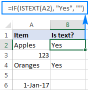
Supposing, you want to insert the word "yes" in column B if a cell in column A contains text. To have it done, put the following formula in B2:
=IF(ISTEXT(A2), "Yes", "")
If cell contains number, then
In a similar fashion, you can identify cells with numeric values (numbers and dates). For this, use the IF function together with ISNUMBER:
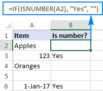
The following formula returns "yes" in column B if a corresponding cell in column A contains any number:
=IF(ISNUMBER(A2), "Yes", "")
If cell contains specific text
Finding cells containing certain text (or numbers or dates) is easy. You write a regular IF formula that checks whether a target cell contains the desired text, and type the text to return in the value_if_true argument.
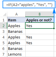
For example, to find out if cell A2 contains "apples", use this formula:
=IF(A2="apples", "Yes", "")
If cell does not contain specific text
If you are looking for the opposite result, i.e. return some value to another column if a target cell does not contain the specified text ("apples"), then do one of the following.
Supply an empty string ("") in the value_if_true argument, and text to return in the value_if_false argument:
=IF(A2="apples", "", "Not apples")
Or, put the "not equal to" operator in logical_test and text to return in value_if_true:
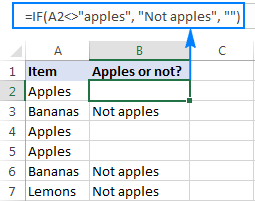
=IF(A2<>"apples", "Not apples", "")
Either way, the formula will produce this result:
If cell contains text: case-sensitive formula
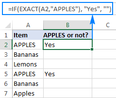
To force your formula to distinguish between uppercase and lowercase characters, use the EXACT function that checks whether two text strings are exactly equal, including the letter case:
=IF(EXACT(A2,"APPLES"), "Yes", "")
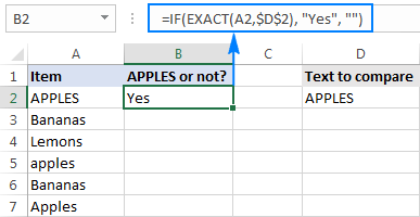
You can also input the model text string in some cell (say in C1), fix the cell reference with the $ sign ($C$1), and compare the target cell with that cell:
=IF(EXACT(A2,$C$1), "Yes", "")
If cell contains specific text string (partial match)
We have finished with trivial tasks and move on to more challenging and interesting ones :) To check if a cell contains specific a given character or substring as part of the cell content, you can use one of these formulas:
Formula 1
Working from the inside out, here is what the formula does:
- The SEARCH function searches for a text string, and if the string is found, returns the position of the first character, the #VALUE! error otherwise.
- The ISNUMBER function checks whether SEARCH succeeded or failed. If SEARCH has returned any number, ISNUMBER returns TRUE. If SEARCH results in an error, ISNUMBER returns FALSE.
- Finally, the IF function returns the specified value for cells that have TRUE in the logical test, an empty string ("") otherwise.
Formula 2
Here, the COUNTIF function finds out how many times a certain text appears in a cell. To count partial matches, you place the wildcard character (*) on both sides of the text. If the count is greater than zero, then IF returns the specified value, otherwise - a blank cell.
And now, let's see how this generic formula works in real-life worksheets.
If cell contains certain text, put a value in another cell
Supposing you have a list of orders in column A and you want to find orders with a specific identifier, say "A-". The task can be accomplished with this formula:
=IF(ISNUMBER(SEARCH("A-", A2)), "Valid", "")
or
=IF(COUNTIF(A2, "*"&"A-"&"*"), "Valid", "")
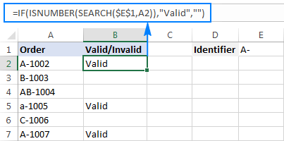
Instead of hardcoding the string in the formula, you can input it in a separate cell (E1), the reference that cell in your formula:
=IF(ISNUMBER(SEARCH($E$1,A2)), "Valid", "")
or
=IF(COUNTIF(A2, "*"&$E$1&"*"), "Valid", "")
For the formula to work correctly, be sure to lock the address of the cell containing the string with the $ sign (absolute cell reference).
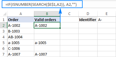
If cell contains specific text, copy it to another column
If you wish to copy the contents of the valid cells somewhere else, simply supply the address of the evaluated cell (A2) in the value_if_true argument:
=IF(ISNUMBER(SEARCH($E$1,A2)),A2,"")
The screenshot below shows the results:
If cell contains specific text: case-sensitive formula
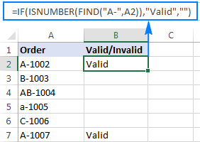
In both of the above examples, the formulas are case-insensitive. In situations when you work with case-sensitive data, use the FIND function instead of SEARCH to distinguish the character case.
For example, the following formula will identify only orders with the uppercase "A-" ignoring lowercase "a-".
=IF(ISNUMBER(FIND("A-",A2)),"Valid","")
If cell contains, then return value – multiple conditions
A single ‘if cell contains’ statement is easy, right? But what if you need to check multiple conditions in the same formula and return different results? That is, if a cell contains some text, then return something, if it contains another text, then return something else, and so on.
To evaluate multiple conditions in a cell, you can use nested "if cell contains" statements. This allows you to create a chain of checks, with each condition leading to a specific result. Here are two generic formulas to achieve this:
Formula 1
Use the COUNTIF function to count how many times a certain text appears in a cell. If the count is greater than zero, then return the corresponding value. Otherwise, check the next condition.
Formula 2
Use the SEARCH function to find the position of a certain text in a cell. If the position is a number, then return the corresponding value. Otherwise, check the next condition.
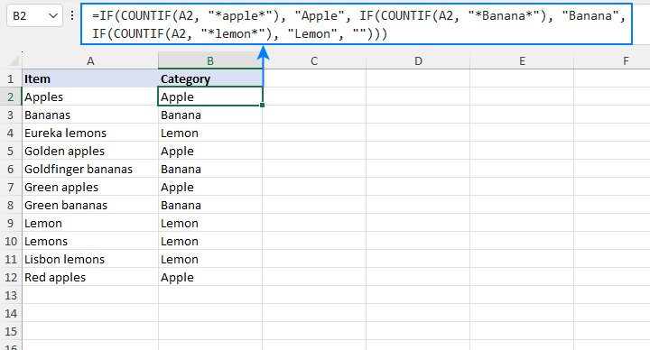
For example, to checks if cell A2 contains "apple", "banana" or "lemon" and return the corresponding name of the fruit in cell B3, you can use one of these formulas:
=IF(COUNTIF(A2, "*apple*"), "Apple", IF(COUNTIF(A2, "*Banana*"), "Banana", IF(COUNTIF(A2, "*lemon*"), "Lemon", "")))
=IF(ISNUMBER(SEARCH("apple", A2)), "Apple", IF(ISNUMBER(SEARCH("banana", A2)), "Banana", IF(ISNUMBER(SEARCH("lemon", A2)), "Lemon", "")))
To fit your specific needs, you can extend the chain of conditions as necessary to handle more cases.
If cell contains one of many text strings (OR logic)
To identify cells containing at least one of many things you are searching for, use one of the following formulas.
IF OR ISNUMBER SEARCH formula
The most obvious approach would be to check for each substring individually and have the OR function return TRUE in the logical test of the IF formula if at least one substring is found:
Supposing you have a list of SKUs in column A and you want to find those that include either "dress" or "skirt". You can have it done by using this formula:
=IF(OR(ISNUMBER(SEARCH("dress",A2)),ISNUMBER(SEARCH("skirt",A2))),"Valid ","")
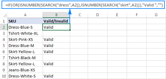
The formula works pretty well for a couple of items, but it's certainly not the way to go if you want to check for many things. In this case, a better approach would be using the SUMPRODUCT function as shown in the next example.
SUMPRODUCT ISNUMBER SEARCH formula
If you are dealing with multiple text strings, searching for each string individually would make your formula too long and difficult to read. A more elegant solution would be embedding the ISNUMBER SEARCH combination into the SUMPRODUCT function, and see if the result is greater than zero:
For example, to find out if A2 contains any of the words input in cells D2:D4, use this formula:
=SUMPRODUCT(--ISNUMBER(SEARCH($D$2:$D$4,A2)))>0
Alternatively, you can create a named range containing the strings to search for, or supply the words directly in the formula:
=SUMPRODUCT(--ISNUMBER(SEARCH({"dress","skirt","jeans"},A2)))>0
Either way, the result will be similar to this:
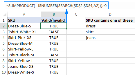
To make the output more user-friendly, you can nest the above formula into the IF function and return your own text instead of the TRUE/FALSE values:
=IF(SUMPRODUCT(--ISNUMBER(SEARCH($D$2:$D$4,A2)))>0, "Valid", "")
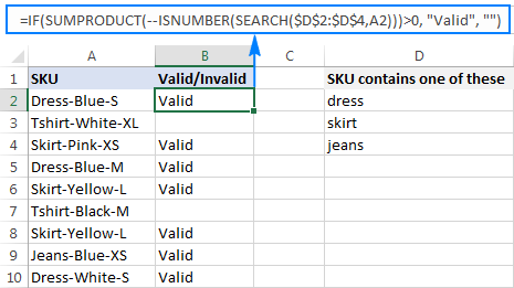
How this formula works
At the core, you use ISNUMBER together with SEARCH as explained in the previous example. In this case, the search results are represented in the form of an array like {TRUE;FALSE;FALSE}. If a cell contains at least one of the specified substrings, there will be TRUE in the array. The double unary operator (--) coerces the TRUE / FALSE values to 1 and 0, respectively, and delivers an array like {1;0;0}. Finally, the SUMPRODUCT function adds up the numbers, and we pick out cells where the result is greater than zero.
If cell contains several strings (AND logic)
In situations when you want to find cells containing all of the specified text strings, use the already familiar ISNUMBER SEARCH combination together with IF AND:
For example, you can find SKUs containing both "dress" and "blue" with this formula:
=IF(AND(ISNUMBER(SEARCH("dress",A2)),ISNUMBER(SEARCH("blue",A2))),"Valid ","")
Or, you can type the strings in separate cells and reference those cells in your formula:
=IF(AND(ISNUMBER(SEARCH($D$2,A2)),ISNUMBER(SEARCH($E$2,A2))),"Valid ","")
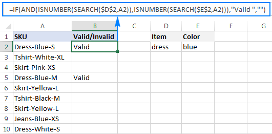
As an alternative solution, you can count the occurrences of each string and check if each count is greater than zero:
=IF(AND(COUNTIF(A2,"*dress*")>0,COUNTIF(A2,"*blue*")>0),"Valid","")
The result will be exactly like shown in the screenshot above.
How to return different results based on cell value
In case you want to compare each cell in the target column against another list of items and return a different value for each match, use one of the following approaches.
Nested IFs
The logic of the nested IF formula is as simple as this: you use a separate IF function to test each condition, and return different values depending on the results of those tests.
Supposing you have a list of items in column A and you want to have their abbreviations in column B. To have it done, use the following formula:
=IF(A2="apple", "Ap", IF(A2="avocado", "Av", IF(A2="banana", "B", IF(A2="lemon", "L", ""))))
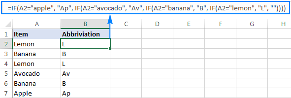
For full details about nested IF's syntax and logic, please see Excel nested IF - multiple conditions in a single formula.
Lookup formula
If you are looking for a more compact and better understandable formula, use the LOOKUP function with lookup and return values supplied as vertical array constants:
For accurate results, be sure to list the lookup values in alphabetical order, from A to Z.
=LOOKUP(A2,{"apple";"avocado";"banana";"lemon"},{"Ap";"Av";"B";"L"})
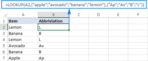
For more information, please see Lookup formula as an alternative to nested IFs.
Vlookup formula
When working with a variable data set, it may be more convenient to input a list of matches in separate cells and retrieve them by using a Vlookup formula, e.g.:
=VLOOKUP(A2, $D$2:$E$5, 2,FALSE )
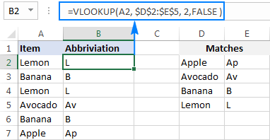
For more information, please see Excel VLOOKUP tutorial for beginners.
This is how you check if a cell contains any value or specific text in Excel. Next week, we are going to continue looking at Excel's If cell contains formulas and learn how to count or sum relevant cells, copy or remove entire rows containing those cells, and more. Please stay tuned!
Practice workbook
Excel If Cell Contains - formula examples (.xlsx file)
 by
by
228 comments
Please could you assist to not allow people to select more than one option. Drop down on both columns to select data or voice. So if a person selects 10GB data, the voice cell must be inactive . if they select voice, data must be inactive
Only Data Only Voice
10GB
125MIN
Hi! I don't really understand what it means for a cell to be inactive. If you want to restrict data entry to individual cells, you may find this tutorial helpful: Data validation in Excel: how to add, use and remove.
Hi! I am attempting to replace the contents of a cell with a number based on whether or not that same number is found in within the cell. Here is the formula I've attempted but I cannot figure out why it is consistently returning a "0" rather than the corresponding number:
=IF(C29(C29, "*1*"), 1, IF(COUNTIF(C29, "*2*"), C29, IF(COUNTIF(C29, "*3*"), 3, IF(COUNTIF(C29, "*4*"), 4, IF(COUNTIF(C29, "*5*"), 5, "")))))
Any help would be greatly appreciated!
Lacy
Hi! Your formula returns nothing because it contains an error. The formula may look like this if you use the COUNTIF function in all conditions:
=IF(COUNTIF(C29, "*1*"), 1, IF(COUNTIF(C29, "*2*"), C29, IF(COUNTIF(C29, "*3*"), 3, IF(COUNTIF(C29, "*4*"), 4, IF(COUNTIF(C29, "*5*"), 5, "")))))
This formula works only with text values. If C29 contains a number, the function returns 0.
It is also unclear what the formula should return if the text contains multiple numbers. For example, "1234".
To offer you a formula, explain your task in more detail.
When A column contains value then B column will write "Yes". When A Column is Blank then B Column "Pending" will be written. When A Column is 0.00 then B Column "NO" will be written.
Use conditional format
Hi! With conditional formatting, you cannot change the value of a cell by condition. Use the guidelines from the article above. This tutorial will also be useful: Nested IF in Excel – formula with multiple conditions. For example:
=IF(A1<>"","Yes",IF(A1=0,"No"))
You can also use the IFS function for multiple conditions:
=IFS(A1<>"","Yes",A1=0,"No")
Hi I have a table where a column captures days overdue (Table2[Ontime / Overdue])
In the same sheet I have a summary at the top showing [P1 etc is the cell it is in]:
[P1] Overdue by 1 Days
[P2] Overdue by 2 Days
[P3] Overdue by 3 Days
[P4] Overdue by 4 Days
[P5] Overdue by 5 Days
[P6] Overdue by >5 Days
(formula in Q1 etc follows =COUNTIF(Table2[Ontime / Overdue],P1) where P1 is a cell with text "Overdue by 1 Days". It is text and number
I am specifically looking to have the [Q6] "Overdue by >5 days" return how many cells have the text showing anything greater than 5 days, though I am having trouble having the formula calculate where it searches the cells (Table2[Ontime / Overdue] for where a number greater than 5 is present.
Any help is much appreciated.
Hi! If I understand your task correctly, you cannot conditionally count text strings that contain different numbers greater than 5. You can only compare to a number, not text.
Thank you for your response, that is good to know. I found a workaround by using another column to use standard count for (Table2[Ontime / Overdue]), then counting how many times that column had instances >5 :)
I have data in one column as bellow
Ram
Ram / Ram
Ram / Ram / Shyam
Shyam / Jay / raj
I want, if only ' Ram' in cell then only Ram
If multiple only ram in cell then multiple ram
If Ram with other then I want answer Ram
with other
If ram not available in cell then answer other
I want formula
Hi! Based on your description, it is hard to completely understand your task. You can count how many times the word "Ram" is found in the text. Split the text into words using the TEXTSPLIT function and count the number of the desired word using the SUMPRODUCT function. You can remove extra spaces with the TRIM function. For example:
=SUMPRODUCT(--(TRIM(TEXTSPLIT(A2,"/"))="Ram"))
Hello - I am sure an easy one but using the formula "=IF(AY11"", "1", "")" ... The resulting retunr of 1, even when formated to number isn't pivotable and is unable to sum the qty of one's on the said Pivot report.
Any ideas anyone would be greatly appreciated.
Hi! Sorry, I have no idea exactly what the task is.
It's hard to tell exactly what you're asking for as it's currently written.
NAME 20 D+ 20 C - 30 B 30 B 23 C 25 C+ - 20 148 C
in the mark list included mark and grade (total mark is 148 with grade)
i want min grade formula in excel
please
Hi! Unfortunately, this information is not enough to give you any advice. You can determine the minimum value with the MIN function. If this does not help, explain the problem in detail.
for eg: five cells contains 1,5,9,3,6. in this we can find the smallest value with the formula
=SMALL(D9:Q9,1)
then, another cells contains A,A+,B,B+. In this format which formula we can?
Hi! I don't understand what you want to do with five numbers and four letters.
Maybe this article will be helpful: MINIFS function in Microsoft Excel – syntax and formula examples
Hello!
I have a question about VLOOPUP(lookup_value, table_array, col_index_num, [range_lookup]). Can we use an array in the "lookup_value"? Something like {"string1";"string2";"string3"}. I just have a long list of complex names, which are sometimes different, but mean the same thing. And in order to match them to the right IDs I need a complex search not out of one word, but multiple. How can I do it? Maybe not VLOOKUP, but something else?
Hi! If you use {"string1"; "string2"; "string3"} as lookup_value, you will get an array of three search results. This formula will return TRUE if at least one value is found:
=SUM(--NOT(ISNA(VLOOKUP({"aaa";"bbb"},B2:C30,2,FALSE))))>0
For more information, read: ISNA function with VLOOKUP.
I hope it’ll be helpful. If something is still unclear, please feel free to ask.
Thanks, but it looks like I phrased the question poorly. I ment if it is possible to have {"string1";"string2";"string3"} as one of the options in the table_array. So that VLOOKUP would have different variations of one name for each ID. Because now when I put a certain name as lookup_value and then put in one cell of the table_array something like {"1_variation";"2_variation" (correct one);"3_variation"}, it gives me N/A, instead of ID, whcih I was looking for. And if I put TRUE as [range_lookup], then sometimes it gives the wrong answer because of alphabetic structure. Sorry for the inconviniece.
Hi! You can write all the variations in one cell as a text string. For example, "1_variation 2_variation 3_variation". Use the TEXTSPLIT function to get an array of variations from this text string. The formula might look something like this:
=SUM(--NOT(ISNA(VLOOKUP(TEXTSPLIT(H1," "),B2:C30,2,FALSE))))>0
I hope it’ll be helpful.
Thank you again! Maybe I am getting something wrong, but your formula has TEXTSPLIT in lookup_value, but variations are inside of the values of table_array. I have multiple versions of one name for each ID in order to cover different spelling and those variations are in the table_array, together with their respective IDs (B2:C30 in your formula). It looks like {"1_variation";"2_variation";"3_variation"} | ID. Lookup_value is just a name that should have an ID from the B2:C30, depending on spelling. Also, your formula returns Bool, but I need ID itself. Is there a way to do it?
Hi! Each of your new questions is different from the previous question. To give you an accurate answer, give an example of the source data and the result you want to get. Describe the problem accurately and in detail.
Hi! I said "I ment if it is possible to have {"string1";"string2";"string3"} as one of the options in the table_array" and "but your formula has TEXTSPLIT in lookup_value, but variations are inside of the values of table_array", so I did't really say anyting different, but if it still is not clear for you, then I will give this example:
| | | |
№| A | B | C | D |
-----------------------------------------------------------------------------------------------------------------------------------------
| | | |
| | | |
1 | 2_var_for_tag1 | VLOOKUP(A1,C1:D10,2, true) -> tag1 | {"1_var_for_tag1";"2_var_for_tag1";"3_var_for_tag1"} | tag1 |
| | | |
2 | 3_var_for_tag2 | VLOOKUP(A1,C1:D10,2, true) -> tag2 | {"1_var_for_tag2";"2_var_for_tag2";"3_var_for_tag2"} | tag2 |
| | | |
3 | 1_var_for_tag3 | VLOOKUP(A1,C1:D10,2, true) -> tag3 | {"1_var_for_tag3";"2_var_for_tag3";"3_var_for_tag3"} | tag3 |
| | | |
...
And so on! Simply adding a new row for each variation won't work, because I have too many rows with data. Hope it will help!
Hi! If I understand your task correctly, try the following formula:
=INDEX($D$1:$D$10,MATCH(TRUE,ISNUMBER(SEARCH(A1,$C$1:$C$10)),0))
For more information, read: How to find substring in Excel
Hi!
I have a fairly specific case and any help would be greatly appreciated. There is a list of signal names that may be slightly different but mean the same thing, for example in column A I have:
Tempreture in the boiler
T in the boiler
Pressure in the tube
Tube pressure
P in the tube
And for each signal there is a list of tags that are always the same, for example they are in column F:
TmBl
PrTb
I need to map different versions of the same signal to its tag in the next column, including the possibility of different spellings. So you should end up with something like this:
Tempreture in the boiler TmBl
T in the boiler TmBl
Pressure in the tube PrTb
Tube pressure PrTb
P in the tube PrTb
I know that I can do this with =IF(COUNTIF(A1;"*Signal1*");"Tag1";IF(COUNTIF(...) ) , but this approach is too long and messy in case I have 50 signals and 150 variations of them. Is there another convenient solution? Maybe I could have some kind of dictionary with keywords for each signal or something like that?
Thank You in advance!
Hi! You can create a table with keywords for each signal. Column A is the signal, column B is the tag. You can use the VLOOKUP or INDEX MATCH function to search for a tag by signal name.
Thank you for the reply, but I am not sure if you can use VLOOKUP or INDEX MATCH with the multiple keywords search. For example, I might have something like:
T after the boiler
Temperature after the boiler
T before the boiler before the valve
T before the boiler after the valve
Which means that if my keyword will be only "T", then I will get only the first option. And if I use such keywords as:
("T", "after", "boiler")
("T", "before", "boiler", "valve")
("T", "before", "boiler", "after", "valve")
Then I will loose the second record where I have "Temprature" instead of "T". So it should be something like:
("T", "Temperature", "after", "boiler")
("T", "before", "boiler", "valve")
("T", "before", "boiler", "after", "valve")
Which means that the formula should be able to take either "T" or "Temperature" AND other words in order to get it right. Is there a way to do this in Excel?
Hi! If each set of keywords will be written in a single cell, then you can use the instructions I recommended. If each keyword will be written in a separate cell in a row, you can use these instructions to search for a tag based on multiple keywords: Excel INDEX MATCH with multiple criteria or How to Vlookup multiple criteria in Excel.
But I recommend writing the key string in a single cell.
I am trying to identify the column # of a cell within a range that contains 2 different strings of text (ordered if necessary), but those are not the only strings within the cell.
e.g. A1 = string 1, string 2, string 3; A2 = string 1, string 4, string 5; A3 = string 3, string 4, string 6
I would like the formula to look at the range A1:A3 and return the position of the cell with string 1 and string 5. As noted above it can be written so they are ordered or unordered, if one is easier than the other.
Hi! If I understand the question correctly, you can determine the position of the cell that has the text strings "string 1" and "string 5" using the MATCH formula. For example:
=MATCH(1,ISNUMBER(SEARCH("string 1",A1:A3)) * ISNUMBER(SEARCH("string 5",A1:A3)),0)
For more information, please read: How to find substring in Excel
I have a sheet with a list of clients and a list of the companies they work for. Is there a way to say if the cell is equal to a company name to then show the employee name on a separate sheet??
Hi! When you want to find a value and get its corresponding value from another column, use these guidelines and examples: Excel VLOOKUP function tutorial with formula examples and INDEX & MATCH in Excel - better alternative to VLOOKUP.
let say i have a cell that contain "Monday morning, tuesday morning" but by using the if function who do i only say yes to one of them which is Monday?
Hi! To determine a partial text match, try this formula:
=IF(ISNUMBER(SEARCH("Monday",A1)),"Yes","")
For more information, please read: How to find substring in Excel
Hi, I have a large set of data with numerous columns, I need a formula that will search if any cells in a row contain a certain key word, if so, I want it to return the FULL contents of that cell.
Example, say I have in row 2, A2 (Star), A3 ($56), A4 (Changed Sales Rep), A5 (3/4/23 updated to cancelled), a6 (Project Name)
And I want the formula to search for 'Cancelled' and return everything in the cell, in this case it would be cell A5 and the return should be '3/4/23 updated to cancelled'
I essentially have a ton of terrible data outputted that cannot easily be delimeted and I need to find the date tied to any substring within the cells that contain the word cancelled.
Thanks in advance.
Hi! Use the INDEX MATCH formula to get a cell with a partial text match. For more information, please read: How to find substring in Excel
Try this formula:
=INDEX(A1:A10,MATCH(TRUE,ISNUMBER(SEARCH("Cancelled",A1:A10)),0))
I hope it’ll be helpful.
Thanks, that did it, very much appreciated!
I'm trying to figure out how to get column c cells which contain various number .ie 20227, 208566, I want column d cells to look for a specific number in C and fill D with the value in A i.e shoe, house etc
Hi! If I understand your task correctly, to find a value in a column and get its corresponding value from another column, this article may be helpful: INDEX & MATCH in Excel.
If the cells in a particular Row (e.g: "m") contains a particular text, then it should be zero , else the amount of another row (e.g: "k") should be shown. Could you please explain?
All the necessary information is in the article above.
okay so i have 261 rows of data in columns a through h. if one of 32 names is in column A2:A261 i need to fill in the data in lines b/row to h/row for example
=IF(A2:A261=A268,B268:H268, IF(A2:A261=A269,B269:H269) ) if i do trhis all the way to =IF(A2:A261,A299,B299:H299) followed by 32 closing brackets will this work to fill my data
Hi! If I understand your task correctly, the following INDEX MATCH formula should work for you:
=INDEX(B268:H299,MATCH(A2,A268:A299,0),)
Try to enter the following formula in cell B2 and then copy it down along the column.
To merge two tables by key columns, you can use the Merge 2 Sheets tool. It is available as a part of our Ultimate Suite for Excel that you can install in a trial mode and check how it works for free.
Good Morning,
I have a slightly different request.
I am trying to write out a sum in one cell, 1+2 for example and in the next cell I want the equation to read =(previous cell) so that it returns the product of the previous equation.
I know I could put each part in a different cell and write the sum as =(first number cell) + (second umber cell) but the list of sums might contain variations or longer sums such as 1*3*(5/4)+7.
Many thanks
Hi! You can only convert text to a formula with VBA.
I have a excel sheet contains petty cash id, discerption and amount. From that each description I want to pop up the result based on the name.
note: Each description is combination of name with voucher number and code.
To ensure clear understanding of your task, can you provide an example of the source data and the desired result you are aiming for?
So I worked out how to make my IF formula work but now I'm facing another issue.
I have in column Q the ages of some people. I need stats on their age.
So in the following columns I have age ranges R=13-25, S=26-35, T=36-64, U=65+
So for the person in Q21 (which is 20) I've got: =IF(AND(Q21>13,Q21<25),"1","0") in cell R21 and in R21 a 1 appears as they're 20 years old. I've made this work for all the people and there are 0's and 1' in the columns to notate their age. Now I want to total how many people are 13-25. My SUM formula isn't working. Is that because It's not reading those cells with the 0's & 1's as numbers because of the IF formula in the cell?
Another SUM formula is able to add up the 1's as a result of an XLOOKUP formula.
I hope this made sense...
Hi! Return a number, not text, to the cell. Then you can summarize it.
=IF(AND(Q2>13,Q21<25),1,0)
Thank you! I didn't know having the number written with quotation marks around it gave it a different value than without. It's working now.
I'm using Excel 2007.
I want the Date of Best Time from all like events displayed in the cell next to Best Time. No luck so far using IF, INDEX(MATCH, VLOOKUP etc., etc. they all give me #Value, False, #N/A, etc. I know barely enough Excel to be dangerous.
I use 12+/- unique MIN(IF functions in Sheet1 to extract the (minimum or fastest) Best Times for each of about 12+/- unique meet events in Sheet2 composed of Date, Col A, Stroke (of 5) Col D, Distance (50, 100,etc. (9)) Col E, Course (Yds/Mtrs) Col F, and Fastest Time (mm:SS.00) Col G, from Sheet2 (Log). Best Time is also posted into Col2 of Sheet1 "Summary." The list is routinely manually updated with new meet info (new rows of event data). The data starts at row 13 and continues to row 154. (Col A of Sheet2 "Log" contains the date of each race event. MIN(IF inserts the Best time in Col B of Sheet1. Sheet1 has other data not associated with this problem.
{=MIN(IF($D$13:$D$154=$D$1,IF($E$13:E$154=$E$1,IF($F$13:$F$154=$F$1,TIMEVALUE($G$13:$G$154)))))}
Specific versions of this function (this one is for a 50 meters freestyle event) work perfectly- I get the Best time . (For events not swum I have entered event rows with temporary data records for each stroke, distance, course, but a 0 in the time column in rows at the bottom of the Sheet2 table . That causes "#Value" to appear in the Best Time column and multiple "#," hash tags in the other derivative cells on Sheet1 which is just fine for me, however, just in case I shorten the ranges to exclude these null records when testing various Date functions.)
Now I want Date of Best time from Sheet2 to appear in Sheet1, Col C. This is the last function I tried: It does not work: (The range (130:144) applies to one section)
{=INDEX(Log!$A$130:$A$144,MATCH($B$63,Log!$G$130:$G$144,))}
Thanks.
Hi! I can't check your formula because I don't have your data. However, I recommend using the [match_type] argument in the MATCH formula:
{=INDEX(Log!$A$130:$A$144,MATCH($B$63,Log!$G$130:$G$144,0))}
For more information, read: How to use MATCH function in Excel.
Thanks.
I still can't get either formula to work. Your formula looks the same as mine, except I forgot the match type. (0) which should mean the look-up array doesn't need to be sorted which mine isn't.
I thought I read that the look-up array must be in or start in the left-most column of the array? T/F? Mine was in Col 7 until I changed it to Col 1 for more tests.
Just in case, I moved and inserted Col 7 (G) before Col 1 (A) on Log (Sheet2) and re-tried INDEX/MATCH and VLOOKUP again. I tried both w/ and w/o SCE
{=INDEX(Log!$B$130:$B$144,MATCH($B$63,Log!$A$130:$A$144,0))}
=VLOOKUP($B$63,Log!$A$130:$B$144,1,FALSE)
Neither worked. "If the lookup value is not found in the lookup array, the #N/A error is returned"- That is exactly what I'm seeing. I verified the look-up value (time) is in the lookup array range and both times are formatted the same- mm:ss.00. What am I missing??
Hi! As I said, I don't have your data to check the formula. Check to see if the time is possibly written as text.
Your wild card example says it will return "B" for anything with "banana" in it, but it returns "L" when it says "yellow banana"
Hi Zac,
You are right - the LOOKUP function does not work correctly with the wildcard character, so I removed that example. Sorry for the confusion.
I have a column with bank statement description in which reference number written at the end of each line and starts with LFT. Is there any why through which i can separate all LFT Number written at the end of each line. Each Line contains different set of long and short description that why i can't use text to column. Let me share two examples of each call .
Example 1: "Transfer Username AHM CABDUL HADI MOHAMMED HAYTHAM AL-TABB LFT23163L52RF "
Example 2: "Transfer ABC travel NAEEM HUSSAIN LFT23163VJTC8G47 "
How can i separate the alphanumeric written at the end and starts with LFT using a formula.
Hi! Find the desired position in the text with the SEARCH function and extract the text string with the MID function.
=MID(A2,SEARCH("lft",A2),20)
Hi all! Incredible post!
I have only 1 question, because I've been trying to solve this issue for hours and I cannot get around it...
I want to be able to do the following:
If cell A1 contains text "ABC" and cell B1 contains text "DEF", result = "100", but if cell A1 contains text "ABC" and cell B1 contains text "GHI", result = "87"; and also, if cell A1 contains text "ABC" and cell B1 doesn't contain "DEF" nor "GHI", result = ""
In "words", this means that I want a cell to reflect a certain result depending on the text content of 2 different cells.
Does anyone have any idea how to do this?
Thanks a bunch.
Best regards,
Charles
Hi! You can find the examples and detailed instructions here: Excel IF statement with multiple conditions. This should solve your task.
If cell contains formula and i want that cell value.
Ex: C2=G2, i want C2 value.
Hi! To check if a cell has the right match use below formula, if it match's it will give "C2" value else return "No Match" where values not match.
=IF(C2=G2,C2,"No Match")
if the value in status column in Dev testing, Sprint planning then i should return a text Development . What formula to use
Can you post your attempts at doing this? What have you done so far to achieve this goal? Please re-check the article above since it covers your case.
Hi,
I would like to use formula =LOOKUP(A2;{"forecast";"sales"};{"F";"S"}) but unfortunately this formula is not working correctly.
My data looks like this (cells contains this kind of information):
JLP ASAF hide sales
forecast
new fabric Forecast
new fabric sales
new fabric still under Development
sales
sales New Fabric
one time only to then be disc
only 126m sold in 2022 avg 2m per week
only 15m sold in 2022 purchased from sales
only 77m sold in 2022
Therefore, if cell contains a word „forecast“, when abbreviation should be „F“. And if cell contains a word „sales“, when abbreviation should be „S“. Unfortunately LOOKUP function is not working. Could you please help me solve this issue. Thanks in advance.
Hi! To determine if a cell has the right word, please read: How to find substring in Excel. You can combine several conditions in a formula using the IFS function.
=IFS(ISNUMBER(SEARCH("sales",A1)),"S", ISNUMBER(SEARCH("forecast",A1)),"F")
Yahooo! Now it's working! Thank you so much!
I want ISBLANK formula before above formula, like=IF(ISBLANK(D2),"Blank",IFS(ISNUMBER(SEARCH("sales",A1)),"S", ISNUMBER(SEARCH("forecast",A1)),"F")....but its not working.
First to find A1 is blank or not, if it is not blank then A3 will be the value of above formula, I mean this formula =IFS(ISNUMBER(SEARCH("sales",A1)),"S", ISNUMBER(SEARCH("forecast",A1)),"F")
can you please help me out
Hi! If you want to check if cell A1 is empty, use ISBLANK(A1) instead of ISBLANK(D2)
I guess, I couldn't explain correctly.
Actually I want 2 formula in a cell. 1st =ISBLANK along with =IFS(ISNUMBER(SEARCH(
First to find A1 is blank or not, if it is not blank then A3 will be the value of | =IFS(ISNUMBER(SEARCH( | formula,
I mean =IF(ISBLANK(A1),"Blank",IFS(ISNUMBER(SEARCH("sales",A1)),"S", ISNUMBER(SEARCH("forecast",A1)),"F")
I’m not sure I got you right since the description you provided is not entirely clear. However, it seems to me that the formula below will work for you:
=IF(ISBLANK(A1),"Blank",IFS(ISNUMBER(SEARCH("sales",A1)),"S", ISNUMBER(SEARCH("forecast",A1)),"F")
This is what I recommended doing in a previous comment.
Hello, I am running Office 365 Excel and in column k I am scanning barcodes (qty up to 1,200), when that number is scanned into a cell in column n what formula can I write to have excel search cells in column b for that same number and then enter a date in the and time in a cell in column k of the same row? I have a code written, when the number is scanned into a cell into column n it finds it and column b and highlights that complete row. Thank you for the help.
Hi! I’m not sure that I got you right, since the description you provided is not entirely clear. Maybe this guide will be helpful: How to insert today date & current time as unchangeable time stamp.
I have a dataset full of dozens of models. The variables used in each model need to be added to one cell with a (+) added between each variable. Not all variables were used in every model, so I need a way to include only the variables and plus sign IF the cell has text (which denotes the variable was used in that particular model). Example of what I mean is below if it shows up properly on the comment page.
A B C D E (output)
Toucan Robin Macaw Toucan + Robin + Macaw
Ostrich Robin Ostrich + Robin
Toucan Ostrich Robin Toucan + Ostrich + Robin
Robin Macaw Robin + Macaw
Thank you for the help!!!
Hi!
If I understand correctly, you want to merge cells with a separator. Use the TEXTJOIN function and this guide: TEXTJOIN function in Excel to merge text from multiple cells.
=TEXTJOIN("+",TRUE,A1:D1)
I have data in "column C" This data contain functions and text as well , Example C1=A1*B1, C2=123, C3=Robert
I need to set the condition in D column as to get only having function in C column, Similarly(Answer result of C1)
I need to set the condition in E column as to get only having number or text in C column(Answer result of C2 and C3
Hope you are clear about the illusturtion and seeking your kind help.
Sunil Pinto.
Hi!
Have you tried the ways described in this blog post? If they don’t work for you, then please describe your task in detail, I’ll try to suggest a solution.
Sir,
Thank you for your prompt response,
I have been gone through your blog
I feel the my requirement is not covered in it.
Actaully I wanted to seggreate the cells with two types
1. Cells Containing:Number and Text or its combination (Example: 123, Sunil, Sunil-123)
2. Cells Containing:Formula or functional result.
Hope you will help me to get resul.
Thank in advance
Regards,
Sunil Pinto.
You can use the ISFORMULA function to identify the cells in which the formula is written.
Hi,
I need to find the text in list of data which contain specific text to return a specific value and am trying to use IF function with combinations of AND and ISNUMBER, SEARCH but it does not return expected result. can you teach me how can I solve this pls?
=IF(AND(ISNUMBER(SEARCH("NC",L4)),AK4="C",H4="WW"),"C-NC",IF(AND(ISNUMBER(SEARCH("SC",L4)),AK4="C",H4="WW"),"C-SC",AK4))
Thank you.
Hi!
Your information is not enough to help. I don't have your data and I don't know what kind of result you want to have.
Hello.
What to do if the "IF" command overwrites cells?
For example, for participant ID N840, age 24 is needed. I am using =IF(A2="N840", "24", ""), and it works well.
However, for a different participant, ID N860, the age needs to be 26. When writing the command, it overwrites the previous one, leaving it blank.
Important to mention that I have multiple data from each participant (longitudinal data).
Thank you very much.
Hi!
I don't really understand what your problem is. Perhaps this article will be helpful to you: How to copy formula in Excel with or without changing references. If this does not help, explain the problem in detail.
Dear alexander,
Thank you for your prompt response. I will try and explain it thoroughly:
I have 20 participants (each has an ID code, e,g., N840), that filled out the same questionnaire over time (meaning, for each participant, I have roughly 16 responses, that is 16 excel rows). The particiapnts filled in their demographic data in a different questionnaire.
I want to assign each participant his age across all of his responses. I am doing the following:
For example, the data for participant N840 is located in excel rows 2, 4, 9, and so on. I am using the following command to enter his age across all rows: IF(B2="N840", "24", ""). It works and fills the column where needed (e.g., rows 2, 9) at the age of 24.
However, when I create a formula for the next participant (A840) in the adjacent row, i.e., IF(B3="A840", "25", ""), it deletes the age data for the previous participants.
I hope it is more clear now.
What can/should I do differently?
Thank you,
Dana
Create a table with 2 columns: ID code and age. You can get the age of each participant from this table using the VLOOKUP function. For example,
=VLOOKUP(A1,Sheet2!A1:B20,2,FALSE)
A1 - participant ID code
For more instructions and examples, see this article: Excel VLOOKUP function tutorial with formula examples.
I hope it’ll be helpful. If something is still unclear, please feel free to ask.
Hi,
I'm trying to find the best formula for my scenario,
I need to search cell B2 - if it contains one word and contains one cell, then result another cell.
Currently, the below formula works
=IF(AND(ISNUMBER(SEARCH("H-Type",B2)),ISNUMBER(SEARCH($AW$2,B2))),$AZ$2,"")
I need to add, if this is false, then continue searching for results with alternative options
Like (SEARCH("P Type",B2)),ISNUMBER(SEARCH($AW$3,B80))),$AZ$3,"") and continue until result is found
Sample/search options for B2:B1840 fields - maybe 30 different text options like "H-Type" or "P-Type"
H-Type® (18"/450mm) X with X and X
P-Type (90"/2200mm) X with X and X
Sample options for AW2:AW24 cells
12"
18"
90" etc
Results - Table(called Sizes) between AZ2:BD24 depending on result of text option
Example. If "H-Type" then result within AZ:2AZ24, if "P-Type" then result within BB2:BB24 etc
Actual value of result will be single numbers between 2 - 20
So, I need to check cell B2 contains "H-Type" and AW2, if yes show value in AZ2, if no check if B2 contains "H-Type" and AW3, if yes show value AZ3, if no continue until a match is found. There should always be a match to one of the combinations between each text and cell option.
or
If B2 contains "H-Type" and AW2 then VLOOKUP(B2,Sizes,4,FALSE))
If B2 contains "P-Type" and AW2 then VLOOKUP(B2,Sizes,6,FALSE))
I hope that all makes sense,
I think this will be way to many conditions for one formula, is this formula even possible?
Thanks,
Hello!
I recommend using the IFS function instead of the IF function for many alternative searches. For more information, read this article: The new Excel IFS function instead of multiple IF.
For example, try this formula:
=IFS(AND(ISNUMBER(SEARCH("H-Type",B2)),ISNUMBER(SEARCH($AW$2,B2))),$AZ$2, AND(ISNUMBER(SEARCH("P Type",B2)),ISNUMBER(SEARCH($AW$3,B80))),$AZ$3)
I hope my advice will help you solve your task.
I am working on a running document. I am attempting to create a formula that will subtract from two cells IF text or a number is present in a different cell. For example if text or a number is present in V3 or U3, then perform E3-D3. My formula looks like:
=if(istext(V3,U3),E3-D3)
But it does not work.
Any ideas?
Hello!
The ISTEXT function only checks the text in the cell, not the number. Try ISBLANK function.
=IF(AND(ISBLANK(U3),ISBLANK(V3)),"",E3-D3)
Hello, I need a help in "improv"ing a formula.
I have something like this in an if: IF(OR(C13="Closed",C13="Dropped",C13="Suspended"), ##DoThis##, ##DoThat## )
Can I rewrite it in a manner where I need to type C13 only once? like..
IF(SOMEFUNCTION(C13,"Closed","Dropped","Suspended"), ##DoThis##, ##DoThat## )
Reason being, there may be another string that might have to be checked for C13, and I am too lazy to type in C13 again ! :)
I am aware that I can probably write it like:
IF(ISNUMBER(FIND(C13,"Closed"&Dropped"&"Suspended")), ##DoThis##, ##DoThat## )
But, is this the only option?
Thank you very much.
Hello!
Instead of a formula
OR(C13="Closed",C13="Dropped",C13="Suspended")
use
OR(C13={"Closed","Dropped","Suspended"})
Hello,
I am trying to add this function; where a particular range of numbers results in a specific text response
for example:
scores in one column within the following ranges (98) will result the following descriptors in the adjacent column (exceptionally low, below average, low average, average, high average, above average, exceptionally high).
how do i write out a command?
Hi!
You can learn more about multiple IF conditions in Excel in this article on our blog: Nested IF in Excel – formula with multiple conditions.
Excellent!
Thank you!!
Hi,
Please help provide the formula if a range of cells contain the letters BR, then I would like the sum of another range of cells of just containing BR to return the value, thank you.
Hello!
To find the sum of the cells by condition, try using the SUMIF function. I hope it’ll be helpful. If this is not what you wanted, please describe the problem in more detail.
Exactly what I needed thank you!
Hi Alexander,
I'm currently using the below formula to extract/filter out data from a master sheet to another sheet, however this gives blank cells/rows in between which I don't want. I tried adding VLOOKUP to the formula but unsuccessful (still noob at using LOOKUP).
=IF(ISNUMBER(SEARCH($I$8,Master!H10)),Master!H10,"")
May I seek your help on how to edit the formula, so that I can have a list of results without blank cells/rows in between please?
Thanks in advance!
Hello!
To get a list of values by condition, I recommend using the FILTER function
For example,
=FILTER(Master!H1:H10,ISNUMBER(SEARCH($I$8,Master!H1:H10)),"")
You can find the examples and detailed instructions here: Excel FILTER function - dynamic filtering with formulas
I have a text string including multiple words and I would like the return value to be different for each IF. For example Statement=send letter with word USD and CAD.If the string includes USD then abbreviate US and if CAD is found then abbreviate CA.
Hi!
To understand what you want to do, give an example of the source data and the desired result.
=IF(ISLBANK(P5),(ISNUMBER(P5), "Done", "Pending"))
I have alredy applied this formula in A5 Cell. So my A5 row is now fill with this formula value. But when my B5 cell value is blank, Then I need to blank also my A5 Cell. How can I applied that with this formula?
HI! I am wondering if you guys can help.. Doing some report for my team
Conditions if scores are from 6.42-7.41 = 5 Coins... if 7.42 - 8;49, 10 coins and if 8.50 - 300, 15 coins.. I used
B22 = 5
B23 = 10
B24 = 15
=IF(C3>=6.42,$B$22,IF(C3>=7.42,$B$23,IF(C3>=8.5,$B$24,)))
C3 is 25.53 but result still is 5. Should be 15. Not sure if there's a mistake with my formula. Thank you.
Hi!
You can find the examples and detailed instructions here: Nested IF in Excel – formula with multiple conditions. Try this formula:
=IF(C3>=8.5,$B$24, IF(C3>=7.42,$B$23, IF(C3>=6.42,$B$22,"")))
If cell G4 contains wording Baseline
Cell H19 mustn't add 5% (Costing)
If cell G4 contains wording Project
Cell H19 must add 5% (Costing)
Hi!
You can find the answer to your question in this article: Nested IF in Excel – formula with multiple conditions.
Need formula in Col B. eg. if B2 contains state listed in D2:D8 & Name of that state should be automatically added there.
| | | |
| A | B | C |
-----------------------------------------------------------------------------------------------------------------------------------------
| | | |
| | | |
| Address | States | Total States |
| | | |
| | | |
| Los Angeles, California, United States, 91311 | California | California |
| | | |
| Santa Clarita, California, United States, 91355-5078 | California | Florida |
| | | |
| Saint Petersburg, Florida, United States, 33701 | Florida | Texas |
| | | |
| Walnut Creek, California, United States, 94596-4410 | California | XYZ |
| | | |
| Roseville, California, United States, 95661 | California | XYZ1 |
| | | |
| Lake Forest, California, United States, 92630-8870 | California | XYZ2 |
| | | |
| Houston, Texas, United States, 92660 | Texas | XYZ3 |
Hi!
Sorry, I do not fully understand the task.
Please clarify your specific problem or provide additional details to highlight exactly what you need. What result do you want to get?
Please advise a number check formula that will yield "if lesser then" in a string scenario (dimensions in a cell) to find out if any of the numbers in their position are lesser then 5.
Cell Example: 11 x 3 x 4
Cell Formula Result: false true true
Hello!
To extract all numbers from text, use a user-defined function RegExpExtract. You can find the examples and detailed instructions here: How to extract substrings in Excel using regular expressions (Regex).
=TEXTJOIN(" ",,(--RegExpExtract(A5,"\d+") < 5))
To combine results in a single cell with a delimiter, use the TEXTJOIN function.
You can also extract all numbers from text using Extract text tool. It is available as a part of our Ultimate Suite for Excel that you can install in a trial mode and check how it works for free.
Hi Dear,
I have an excel file where a cell can contain 2 languages (Arabic and English). Is there a way to highlight which of these cells in the sheet have 2 languages. Also, is there a way to further determine if the English language (word) starts at the beginning of the sentence.
The problem is that we are working on a project to create an app, some sentences should include popular english words followed by arabic words. But whenever the sentence start with english, a problem appears in our user interface. That's why I need to determine which sentences in the cell start with and English word.
Thank you!
Hello!
You can determine the ANSI code of the first character in a text. The ASCII value of the lowercase alphabet is from 97 to 122. And, the ASCII value of the uppercase alphabet is from 65 to 90. To do this, use the CODE function.
=CODE(LEFT(A1,1))
See CODE function example here.
I hope my advice will help you solve your task.
Thank you so much Alexander. This helped me a lot!
Hi, need help with a formula, please:
If cell contains certain text, put a value in another cell: So that would be =IF(ISNUMBER(SEARCH("Sub",A2)),"Approve","")
But, I would like to use such a formula to look for "Sub" in a range of cells, for example, A2:F2 (1st case scenario), and then in a different instance, to look for "Sub" in a group of cells - A2, C2, D2 and G2 (2nd case scenario).
Thank you very much in advance.
Stan
Hello!
Try using the SUM formula to get the search result in a range.
=IF(SUM(--ISNUMBER(SEARCH("Sub",A2:F2))),"Approve","")
I hope it’ll be helpful.
Kind greetings and thank you very much for your kind help / response. I tried the equation that you helped provide above but it still provides a blank response, even when one of the cells contains "Sub".
In this case, I'm trying to approve the the row #3 because one of the cells from C3 to G3, in this case E3, contains the string "Sub".
A B C D E F G H
1 Alt ID Plans CovA CovB CovC CovD CovE Approval
2 101020 Pol3 Plan11 Coord2e
3 907030 Pol Sub5a Alt24
4 805050
5 778050 Plan88 Sub7d Coord2
6 232520 Sub4 ALt4 Plan6
7 357031 Plan2d Sub7e
So, I used =IF(SUM(--ISNUMBER(SEARCH("Sub",C3:G3))),"Approve","") but it still gives a blank response.
Thank you again, in advance.
Stan
Hi!
I have used your data. The formula works.
Hi, thank you very much for your kind help. I read one of your blogs on Excel ISNUMBER function with formula examples, under conditioning with SUMPRODUCT and it helped.
The equation I'm using now is =IF(SUMPRODUCT(--ISNUMBER(SEARCH("Sub",C3:G3))),"Approve","") and it is helping with what I needed to do.
Again, your very kind help is much appreciated.
Hello!
You didn't specify this, but I'm assuming you're working with Excel 2019 or 2016. The formula returns an array that needs to be summed. In Excel 365, you do not need to do this.
Sorry about that; and yes, I'm working with Excel 2019.
Again, I thank you.
Best regards,
Stan
Hi Alexander,
I am new to extended formulas. I usually manage with Vlook Up and Pivots. I am trying to show value of cell B2 in cell C2, if Text in Cell A2 is specific and if not, then value in Cell C2 must reflect "0" / zero. Likewise, for Row no.s 3, 4, 5, ....
Eg., A2 value is "Opening Balance", B2 value is "100" then C2 must reflect the value of Cell B2 i.e., "100". But if A2 value is NOT "Opening Balance" then C2 must reflect "0" / zero in numerical value. Please help me.
A B C D E F
Transactions Amount Opening Balance Invoice Debit Note Receipt
1 Opening Balance 100.00 100.00 0 0 0
2 Invoice 248.00 0 248.00 0 0
3 Debit Note 10.00 0 0 10.00 0
4 Receipt 238.00 0 0 0 238.00
Thanks,
Anand
Hello!
For your task, you can use the IF function.
IF(A2="Opening Balance", B2, 0)
If the suggested formula doesn't work for your case, feel free to describe it in detail.
Great information. Is it possible to put a formula in a cell that tests a different cell and places text in a 3rd cell ?
Example: Formula is in cell E1, testing cell A1 is equal to "Test", setting cell B1 equal to "Yes"
Cell B1 has other text in it until cell A1 has been changed to "Test" manually.
If, Then , Else structure but being able to specify the cells for the then and Else output.
I used this structure but can not specify a target cell
Cell B1 is =IF(ISNUMBER(SEARCH("Test,A1)),"Yes","No") will set B1 to Yes or No
but wish to add target cells for results:
Formula is in cell E1 =IF(ISNUMBER(SEARCH("Test,A1)),("Yes",B1),("No",C1)) Target cells are B1 and C1
I know how to do it in Macro but then need to run the macro. I wanted it to happen without running or adding macro.
Thanks,
Vin
Hi!
It has already been written many times in this blog that an Excel formula can only change the value of the cell in which it is written. For all other tasks, use VBA.
Hello, I would like to seek help. If a cell has a text value: then perform another formula else blank
Hi!
To check if a value is text, use the Excel IF ISTEXT formula.
I know how to count a series of keywords in Excel. I use this formula: =SUMPRODUCT(--ISNUMBER(SEARCH($CE$2:$CE$43,(G2:AP2))))
However, what would be the Excel formula if I want to count the number of keywords that exist only within +/-3 words around "risk" in the selected rows?
Consider this sentence: "Political uncertainty generates economic risk which stagnates economic activities." If my keywords are "political", "uncertainty", "stagnates", and economic", the total number of keywords within +/- 3 words around "risk" will be 3, i.e., "uncertainty", "stagnates", and "economic". "political" will be excluded since it is out of range.
IF the cell contains numbers and characters and without numbers , how can i filter only character cells please help me
Hello!
I recommend using a custom function REGEXMATCH. You can find the examples and detailed instructions here: How to use regex to match strings in Excel. You can filter on the TRUE value that this function will return.