The tutorial shows how to create multiple IF statements in Excel with AND as well as OR logic. Also, you will learn how to use IF together with other Excel functions.
In the first part of our Excel IF tutorial, we looked at how to construct a simple IF statement with one condition for text, numbers, dates, blanks and non-blanks. For powerful data analysis, however, you may often need to evaluate multiple conditions at a time. The below formula examples will show you the most effective ways to do this.
How to use IF function with multiple conditions
In essence, there are two types of the IF formula with multiple criteria based on the AND / OR logic. Consequently, in the logical test of your IF formula, you should use one of these functions:
- AND function - returns TRUE if all the conditions are met; FALSE otherwise.
- OR function - returns TRUE if any single condition is met; FALSE otherwise.
To better illustrate the point, let's investigate some real-life formulas examples.
Excel IF statement with multiple conditions (AND logic)
The generic formula of Excel IF with two or more conditions is this:
Translated into a human language, the formula says: If condition 1 is true AND condition 2 is true, return value_if_true; else return value_if_false.
Suppose you have a table listing the scores of two tests in columns B and C. To pass the final exam, a student must have both scores greater than 50.
For the logical test, you use the following AND statement: AND(B2>50, C2>50)
If both conditions are true, the formula will return "Pass"; if any condition is false - "Fail".
=IF(AND(B2>50, B2>50), "Pass", "Fail")
Easy, isn't it? The screenshot below proves that our Excel IF /AND formula works right:

In a similar manner, you can use the Excel IF function with multiple text conditions.
For instance, to output "Good" if both B2 and C2 are greater than 50, "Bad" otherwise, the formula is:
=IF(AND(B2="pass", C2="pass"), "Good!", "Bad")
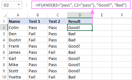
Important note! The AND function checks all the conditions, even if the already tested one(s) evaluated to FALSE. Such behavior is a bit unusual since in most of programming languages, subsequent conditions are not tested if any of the previous tests has returned FALSE.
In practice, a seemingly correct IF statement may result in an error because of this specificity. For example, the below formula would return #DIV/0! ("divide by zero" error) if cell A2 is equal to 0:
=IF(AND(A2<>0, (1/A2)>0.5),"Good", "Bad")
The avoid this, you should use a nested IF function:
=IF(A2<>0, IF((1/A2)>0.5, "Good", "Bad"), "Bad")
For more information, please see IF AND formula in Excel.
Excel IF function with multiple conditions (OR logic)
To do one thing if any condition is met, otherwise do something else, use this combination of the IF and OR functions:
The difference from the IF / AND formula discussed above is that Excel returns TRUE if any of the specified conditions is true.
So, if in the previous formula, we use OR instead of AND:
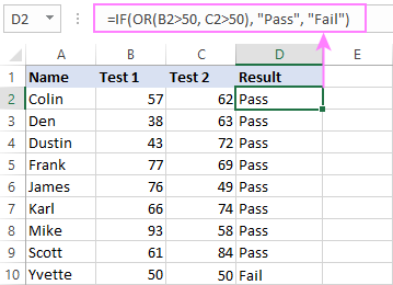
=IF(OR(B2>50, B2>50), "Pass", "Fail")
Then anyone who has more than 50 points in either exam will get "Pass" in column D. With such conditions, our students have a better chance to pass the final exam (Yvette being particularly unlucky failing by just 1 point :)
Tip. In case you are creating a multiple IF statement with text and testing a value in one cell with the OR logic (i.e. a cell can be "this" or "that"), then you can build a more compact formula using an array constant.
For example, to mark a sale as "closed" if cell B2 is either "delivered" or "paid", the formula is:
=IF(OR(B2={"delivered", "paid"}), "Closed", "")
More formula examples can be found in Excel IF OR function.
IF with multiple AND & OR statements
If your task requires evaluating several sets of multiple conditions, you will have to utilize both AND & OR functions at a time.
In our sample table, suppose you have the following criteria for checking the exam results:
- Condition 1: exam1>50 and exam2>50
- Condition 2: exam1>40 and exam2>60
If either of the conditions is met, the final exam is deemed passed.
At first sight, the formula seems a little tricky, but in fact it is not! You just express each of the above conditions as an AND statement and nest them in the OR function (since it's not necessary to meet both conditions, either will suffice):
OR(AND(B2>50, C2>50), AND(B2>40, C2>60)
Then, use the OR function for the logical test of IF and supply the desired value_if_true and value_if_false values. As the result, you get the following IF formula with multiple AND / OR conditions:
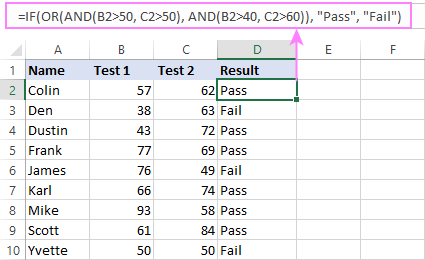
=IF(OR(AND(B2>50, C2>50), AND(B2>40, C2>60), "Pass", "Fail")
The screenshot below indicates that we've done the formula right:
Naturally, you are not limited to using only two AND/OR functions in your IF formulas. You can use as many of them as your business logic requires, provided that:
- In Excel 2007 and higher, you have no more than 255 arguments, and the total length of the IF formula does not exceed 8,192 characters.
- In Excel 2003 and lower, there are no more than 30 arguments, and the total length of your IF formula does not exceed 1,024 characters.
Nested IF statement to check multiple logical tests
If you want to evaluate multiple logical tests within a single formula, then you can nest several functions one into another. Such functions are called nested IF functions. They prove particularly useful when you wish to return different values depending on the logical tests' results.
Here's a typical example: suppose you want to qualify the students' achievements as "Good", "Satisfactory" and "Poor" based on the following scores:
- Good: 60 or more (>=60)
- Satisfactory: between 40 and 60 (>40 and <60)
- Poor: 40 or less (<=40)
Before writing a formula, consider the order of functions you are going to nest. Excel will evaluate the logical tests in the order they appear in the formula. Once a condition evaluates to TRUE, the subsequent conditions are not tested, meaning the formula stops after the first TRUE result.
In our case, the functions are arranged from largest to smallest:
=IF(B2>=60, "Good", IF(B2>40, "Satisfactory", "Poor"))
Naturally, you can nest more functions if needed (up to 64 in modern versions).

For more information, please see How to use multiple nested IF statements in Excel.
Excel IF array formula with multiple conditions
Another way to get an Excel IF to test multiple conditions is by using an array formula.
To evaluate conditions with the AND logic, use the asterisk:
To test conditions with the OR logic, use the plus sign:
To complete an array formula correctly, press the Ctrl + Shift + Enter keys together. In Excel 365 and Excel 2021, this also works as a regular formula due to support for dynamic arrays.
For example, to get "Pass" if both B2 and C2 are greater than 50, the formula is:
=IF((B2>50) * (C2>50), "Pass", "Fail")

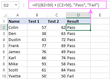
In my Excel 365, a normal formula works just fine (as you can see in the screenshots above). In Excel 2019 and lower, remember to make it an array formula by using the Ctrl + Shift + Enter shortcut.
To evaluate multiple conditions with the OR logic, the formula is:
=IF((B2>50) + (C2>50), "Pass", "Fail")
Using IF together with other functions
This section explains how to use IF in combination with other Excel functions and what benefits this gives to you.
Example 1. If #N/A error in VLOOKUP
When VLOOKUP or other lookup function cannot find something, it returns a #N/A error. To make your tables look nicer, you can return zero, blank, or specific text if #N/A. For this, use this generic formula:
For example:
If #N/A return 0:
If the lookup value in E1 is not found, the formula returns zero.
=IF(ISNA(VLOOKUP(E1, A2:B10, 2,FALSE )), 0, VLOOKUP(E1, A2:B10, 2, FALSE))
If #N/A return blank:
If the lookup value is not found, the formula returns nothing (an empty string).
=IF(ISNA(VLOOKUP(E1, A2:B10, 2,FALSE )), "", VLOOKUP(E1, A2:B10, 2, FALSE))
If #N/A return certain text:
If the lookup value is not found, the formula returns specific text.
=IF(ISNA(VLOOKUP(E1, A2:B10, 2,FALSE )), "Not found", VLOOKUP(E1, A2:B10, 2, FALSE))

For more formula examples, please see VLOOKUP with IF statement in Excel.
Example 2. IF with SUM, AVERAGE, MIN and MAX functions
To sum cell values based on certain criteria, Excel provides the SUMIF and SUMIFS functions.
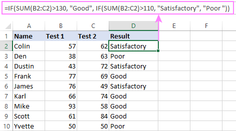
In some situations, your business logic may require including the SUM function in the logical test of IF. For example, to return different text labels depending on the sum of the values in B2 and C2, the formula is:
=IF(SUM(B2:C2)>130, "Good", IF(SUM(B2:C2)>110, "Satisfactory", "Poor"))
If the sum is greater than 130, the result is "good"; if greater than 110 – "satisfactory', if 110 or lower – "poor".
In a similar fashion, you can embed the AVERAGE function in the logical test of IF and return different labels based on the average score:
=IF(AVERAGE(B2:C2)>65, "Good", IF(AVERAGE(B2:C2)>55, "Satisfactory", "Poor"))
Assuming the total score is in column D, you can identify the highest and lowest values with the help of the MAX and MIN functions:
=IF(D2=MAX($D$2:$D$10), "Best result", "")
=IF(D2=MAX($D$2:$D$10), "Best result", "")
To have both labels in one column, nest the above functions one into another:
=IF(D2=MAX($D$2:$D$10), "Best result", IF(D2=MIN($D$2:$D$10), "Worst result", ""))

Likewise, you can use IF together with your custom functions. For example, you can combine it with GetCellColor or GetCellFontColor to return different results based on a cell color.
In addition, Excel provides a number of functions to calculate data based on conditions. For detailed formula examples, please check out the following tutorials:
Example 3. IF with ISNUMBER, ISTEXT and ISBLANK
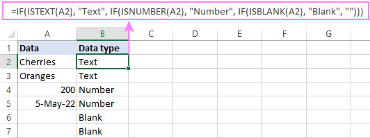
To identify text, numbers and blank cells, Microsoft Excel provides special functions such as ISTEXT, ISNUMBER and ISBLANK. By placing them in the logical tests of three nested IF statements, you can identify all different data types in one go:
=IF(ISTEXT(A2), "Text", IF(ISNUMBER(A2), "Number", IF(ISBLANK(A2), "Blank", "")))
Example 4. IF and CONCATENATE
To output the result of IF and some text into one cell, use the CONCATENATE or CONCAT (in Excel 2016 - 365) and IF functions together. For example:
=CONCATENATE("You performed ", IF(B1>100,"fantastic!", IF(B1>50, "well", "poor")))
=CONCAT("You performed ", IF(B1>100,"fantastic!", IF(B1>50, "well", "poor")))
Looking at the screenshot below, you'll hardly need any explanation of what the formula does:

IF ISERROR / ISNA formula in Excel
The modern versions of Excel have special functions to trap errors and replace them with another calculation or predefined value - IFERROR (in Excel 2007 and later) and IFNA (in Excel 2013 and later). In earlier Excel versions, you can use the IF ISERROR and IF ISNA combinations instead.
The difference is that IFERROR and ISERROR handle all possible Excel errors, including #VALUE!, #N/A, #NAME?, #REF!, #NUM!, #DIV/0!, and #NULL!. While IFNA and ISNA specialize solely in #N/A errors.
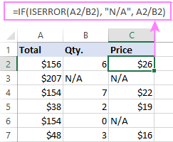
For example, to replace the "divide by zero" error (#DIV/0!) with your custom text, you can use the following formula:
=IF(ISERROR(A2/B2), "N/A", A2/B2)
And that's all I have to say about using the IF function in Excel. I thank you for reading and hope to see you on our blog next week!
Practice workbook for download
Excel IF multiple criteria - examples (.xlsx file)
 by
by
4506 comments
Hello, I am looking for help to write a formula based on nursing staffing.
Here is the example I need help with creating a formula for in a spreadsheet
The census is 30 and there are 5 registered nurses and 1 licensed practical nurse working … the formula I need help with would calculate 1 nurse and 1 licensed practical nurse work together take 9 patients. (The census of 30 patients minus the 9 patients the 2 staff take is 21). Therefore the remaining 4 registered nurses are split between the remaining 21 patients (so 3 nurses have 5 patients and 1 nurse would have 6 patients).
My spreadsheet has one column (cell) for the census, 1 cell for RN, and 1 cell for LPN.
I need to be able to calculate the ratio for this rule with an if function, because there is not always an LPN scheduled to work, so when a 1 is entered into the LPN cell, it should count a RN & LPN working together with 9 patients. (If no LPN is working, the RNs are divided among the unit census).
If someone can please help me, I have tried looking up help for this! I am not sure that an “if” rule is correct or how to proceed figuring this out.
Hi! Your request goes beyond the advice we provide on this blog. This is a complex solution that cannot be found with a single formula. If you have a specific question about the operation of a function or formula, I will try to answer it.
I have 3 criteria and 9 condition with same criteria in different column for incentive calculation. then which formula we can try to do smooth work.
Exp.:- If quarterly target is 5 lakhs, and achievement is 5.2 lakhs (104%
achievement) then MR will be eligible for Group B incentive that is 1.20% of the
quarterly sale that is 6240 Rs.
In that case we have 3 group 3 different condition and in three Group we have another condition with achievement. so pls suggest
Achievement Terms Group A Group B Group C
2.5 L
95-99.99% 0.50% 0.60% 0.75%
100-104.99% 1% 1.20% 1.50%
105-109.99% 1.25% 1.40% 1.75%
>110% 1.50% 1.80% 2%
Hi! You can create many conditions for IF function as described in this guide: Nested IF in Excel – formula with multiple conditions. You can also use the information and examples from the article above. Create a separate formula for each group. Or you can combine these formulas if you make a group selection and then specify a calculation for each group. For example:
=IF(G1="Group A",IF(AND(H1>95%,H1<99.99%),0.5%, IF(AND(H1>100%,H1<104.99%),1%,"")), IF(G1="Group B", IF(AND(H1>95%,H1<99.99%),0.6%, IF(AND(H1>100%,H1<104.99%),1.2%,""))))
Hello, thanks for the great work
I have an exercise please and I need help to apply a discaount on excel.
Regarding the discounts to apply:
6% if the customer is a wholesaler and bought more than € 10,000 in goods
3% if the customer is an individual and bought more than € 10,000 in merchants
0% if it is a retailer or if the customer bought less than € 10,000 while being wholesaler/individual.
Which function can I use please?
Hello! All the necessary information is in the article above. For multiple conditions, you can use a nested IF function. Read the following paragraph of the article above: Multiple nested IF statements. You can also find useful information in this article: Nested IF in Excel – formula with multiple conditions.
If each criterion of a nested IF function includes two conditions, you can use the AND function for those conditions as described in the paragraph above: Multiple AND conditions, and in this article: Multiple IF AND statements in Excel.
This should solve your task.
Looking to do something similar
Where multiple duplicates of transactions but need it to group the customers then show the first payment is declined and last payment is approved.
What would be the best way to complete this task ?
Columns
Decision = Decline or approves
Date
Customer email
Count of orders
Hi! Based on your description, it is hard to completely understand your task. However, I’ll try to guess and offer you the following guide: How to find duplicates in Excel: identify, highlight, count, filter.
Hi, need help with these:
Between 94.99% to 85% = 5
95.00% - 99.99% = 4
100.00% - 104.99% = 3
105.00% - 109.99% = 2
110% and above | Below 85% = 1
Hi! The answer to your question can be found in this article: Nested IF in Excel – formula with multiple conditions.
hi,
if one cell value equal or less than 14, is answer is "0"
if one cell value more than 14 is answer their value actual.
Hi! The answer to your question can be found in this guide: IF formula for numbers.
Formula for multiple LEFT Function in referencing to 1 cell only. The results either should be 2 digits,3 digits, 4 digits and 5 digits/
Hi! Your question is not clear. I think you can solve the problem yourself if you use this manual: Excel LEFT function with formula examples. If you can't do this, give an example of source data and desired results.
Hi guys need help.
Im looking what function to use
If A1 = “5x9” it should follow a 30 mins break and if more than 30 mins it should result to 1. if not, 0.
Then, if A1= “4x11” it should follow a 40 mins break and if more than 40 mins it should result to 1. if not, 0.
Hi! For multiple conditions you can use the nested IF function. I can't recommend you a formula, as not all your conditions are clear to me. For example "if more than 30 mins".
Please suggest a formula for below conditions
up to 150 show result "3"
151 to 1200 show result "5"
1201 to 35000 show result "8"
Hi! We have a special tutorial on this. Please see: Nested IF in Excel – formula with multiple conditions.
Hi,
I wanna create a formula within the IF function. I have got two variables in a list, and I want a mathematical formula to be applied based on the selection from the list.
Hi! To perform calculations depending on the value of the variable selected in the list, use the recommendations in the article above and the easier examples in this manual: Excel nested IF statement - multiple conditions in a single formula.
I want create formula
if A1 is less then 100k then result willbe zero, if A1 greater than 100k & less then result willbe A1*2%
If A1 greater than 200k & less than 500k then result will A1*5%
Hi! The answer to your question can be found in the article above in this section: Multiple nested IF statements. You can also find useful information in this article: Nested IF in Excel – formula with multiple conditions.
thank you so much sir, verry helpful
Trying to get a rolling calculation for 2 different factors.
To calculate data from column b2 to u2.
If a number is greater than 0, want the number 25 to be added for each cell and have total shown in cell v2.
Purpose is to capture total fixed number of “items” looked at. What is entered is number of “items” broken.
The average is done in a different cell based off of total number of items looked at.
Hi! If I understand your task correctly, this guide may be helpful: Excel average without zeros.
I have 3 variable. In all 3 variable the value is present in only one variable so after making the 4 variable the data should come from there.
Hi! To extract the value from the cell that contains data, you can use the following formula in a fourth cell (e.g., D1):
=IF(A1<>"", A1, IF(B1<>"", B1, C1))
Read more: Nested IF in Excel – formula with multiple conditions.
i am traying to write in if formula that a cell b7
if b7 is less than or equal to 50, value is 7
if b7 is greater than 50,but less than and equal to 150, value is 19
if b7 is greater than 150 but less than and equal to 400, value is 37
i want to apply this formula for a cell
Hi! You can find the answer in the first section of this article: Nested IF in Excel – formula with multiple conditions.
I am trying to insert IF where the following:
If C2 = "Closed",(E2*M13) and if C2 = "PAI",(E2*M9) and if C2 = TRAY,(E2*M7) and so on...
So if my c reads as closed, the cell calculates a value by taking the total in E and multiplying by % in M and if my c reads as PAI, it calculates the value by taking total in E and multiplying by corresponding % in M and so on.
I can't seem to add arguments after the first. I only have =IF(C2="closed",(CurrentWIP!E2*Sheet1!$B$18)) which works, looking only at 1 criteria. How do I add the same formula with different cells after the last ))
Hi! You can find the examples and detailed instructions here: Nested IF in Excel – formula with multiple conditions. For example:
=IF(C2="Closed",E2*M13,IF(C2="PAI",E2*M9,""))
Hi, I have cell D88 with text "DCC Incentive|MASTERCARD DCC1080225681".
In cell E88 and F88 I have Debit & Credit amount respectively. For this transaction, the amount is in Credit amount column USD8. I want to put 2 condition in cell J88, 1st : if 1st 13 left character is "DCC Incentive" and if F88>0, the final result should be a "Deposit"or "Payment" if false.
can you help which if formula to apply here?
Hi! If I understand your task correctly, the following formula should work for you:
=IF(AND(LEFT(D88,13)="DCC Incentive", F88>0), "Deposit","Payment")
Use the LEFT function to extract the characters from cell D88. Compare the result with the sample text. Depending on the conditions, use IF AND functions to write the final result.
I have a table with columns A through to Q.
I want a formula in column E that looks into B and if it finds "prof services" it always returns a 0, but if it doesn't it will multiple columns C x D. Thats all pretty simple but I also want other conditions to apply. If J states "No" then I want to multiple (C X D) x 0.8 unless Q contains "Partner". If "Partner" is returned I just want C X D.
The following formula is in Column E
=IFERROR(IF($B14="Prof Services",0,IF(Q14="Telstra",D14,IF(J14=”No”,$D14*0.8,D14)))," ")
The output I am hoping to get:
If B14 = "Prof Services" then I want 0 in E14
But if B14 = anything other than "Prof Services" then I want the value of D14 in E14 unless J14 has "No". In that case I want the value of D14 multiplied by 0.8
But with one other condition, and that is if "Telstra" is in cell Q14, then just show D14
Hi! The answer to your question can be found in article above and in this article: Nested IF in Excel – formula with multiple conditions. I can't offer you a formula as your description of the conditions is not very clear.
Thanks Alex, Nested IF worked perfectly, once I worked out the logic. Thanks again
I'm trying to write a formula for this scenario:
Cell A2
Cell B2
Cell C2
If Cell A2 is equal to zero, Cell A2 - Cell B2 = Cell C2
If Cell A2 is > zero, Cell A2 - Cell B2 = Cell C2
=IF(A2=0,A2-B2,IF(A2>0,A2-B2,""))
This will only shows result in Cell C2 once figure is key in. How do I make the same thing if Cell A2 is zero?
I am not sure I fully understand what you mean. The answer to your question is already in your formula. I don't really understand why you need two conditions with the same result. One condition is enough.
=IF(A2>=0,A2-B2,"")
I am having trouble combining a CONCATENATION formula with an IF statement.
This works as expected, both when A22 exists and when it doesn't: =IF(A22,"Hello","")
This works as expected: =CONCATENATE(TEXT(A22,"ddd. "),TEXT(C22,"mmm. dd"))
But this works as expected only when A22 exists. If A22 is empty I get "FALSE" not the " " I want: =IF(A22,CONCATENATE(TEXT(A23,"ddd. "),TEXT(C23,"mmm. dd")," "))
I suspect that the commas in the CONCATENATION statement are confusing the IF formula. But I've tried numerous additions of parentheses (to solate the CONCATENATION elements from IF) and Excel only balks.
Any thoughts?
Hi! If I understand your task correctly, the following formula should work for you:
=IF(A22,CONCATENATE(TEXT(A23,"ddd. "),TEXT(C23,"mmm. dd"))," ")
You're right. It does. Such a simple fix. All in the placement of the parentheses. I thought I had tried the very same placement at least twice before and gotten errors. But now it works. Thanks very much.
Excel wizards of this world, please help!
I'm trying to write a VLOOKUP formula that will give me a "-" in return when the value is either not found or zero, and the actual value when it was found. I've tried several approaches, but I can't get it to work. My latest attempt was this one:
=IF(OR(VLOOKUP(B1;location;5;FALSE)=0);(IFERROR(VLOOKUP(B1;location;5;FALSE))));"0";(VLOOKUP(B1;location;5;FALSE))
Thanks!
Hi! To replace the #N/A error with a value and use the second condition, apply a nested IF. For example:
=IF(ISNA(VLOOKUP(B1,C1:G15,5,FALSE)),"-", IF(VLOOKUP(B1,C1:G15,5,FALSE),"-", VLOOKUP(B1,C1:G15,5,FALSE)))
Read more: Nested IF in Excel – formula with multiple conditions.
Hi, I am trying to find a formula for the following logic. thank you in advance for helping out. If in Cell B1 there is one of 3 txt1, txt2, tx3, then it should return a value of -10 days prior to date from Cell A1.
Thank you
Hi! Have you tried the ways described in this blog post? It contains answers to your question. You could also find the solution in this article: Excel IF OR statement with formula examples. For example:
=IF(OR(B1="txt1",B1="txt2"),A1-10,"")
I trying to work on If Column D = Y, Column A to apply formula figure 1.0x130% and if D=N column A should remain as 1.0
Hi! You can find the examples and detailed instructions here: Nested IF in Excel – formula with multiple conditions.
I am trying to reference a table on a different sheet in a workbook and populate a Yes or no in a cell if two criteria are true in that data set. Which Function do I use for that?
Hi! Unfortunately, this information is not enough to give you any advice. If the information from the article above is not enough to solve your problem, I need to know more details about your task to help you.