The tutorial explains the syntax of the Excel FIND and SEARCH functions and provides formula examples of advanced non-trivial uses.
In the last article, we covered the basics of the Excel Find and Replace dialog. In many situations, however, you may want Excel to find and extract data from other cells automatically based on your criteria. So, let's have a closer look at what the Excel search functions have to offer.
Excel FIND function
The FIND function in Excel is used to return the position of a specific character or substring within a text string.
The syntax of the Excel Find function is as follows:
The first 2 arguments are required, the last one is optional.
- Find_text - the character or substring you want to find.
- Within_text - the text string to be searched within. Usually it's supplied as a cell reference, but you can also type the string directly in the formula.
- Start_num - an optional argument that specifies from which character the search shall begin. If omitted, the search starts from the 1st character of the within_text string.
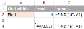
If the FIND function does not find the find_text character(s), a #VALUE! error is returned.
For example, the formula =FIND("d", "find") returns 4 because "d" is the 4th letter in the word "find". The formula =FIND("a", "find") returns an error because there is no "a" in "find".
Excel FIND function - things to remember!
To correctly use a FIND formula in Excel, keep in mind the following simple facts:
- The FIND function is case sensitive. If you are looking for a case-insensitive match, use the SEARCH function.
- The FIND function in Excel does not allow using wildcard characters.
- If the find_text argument contains several characters, the FIND function returns the position of the first character. For example, the formula FIND("ap","happy") returns 2 because "a" in the 2nd letter in the word "happy".
- If within_text contains several occurrences of find_text, the first occurrence is returned. For example, FIND("l", "hello") returns 3, which is the position of the first "l" character in the word "hello".
- If find_text is an empty string "", the Excel FIND formula returns the first character in the search string.
- The Excel FIND function returns the #VALUE! error if any of the following occurs:
- Find_text does not exist in within_text.
- Start_num contains more characters than within_text.
- Start_num is 0 (zero) or a negative number.
Excel SEARCH function
The SEARCH function in Excel is very similar to FIND in that it also returns the location of a substring in a text string. Is syntax and arguments are akin to those of FIND:
Unlike FIND, the SEARCH function is case-insensitive and it allows using the wildcard characters, as demonstrated in the following example.
And here's a couple of basic Excel SEARCH formulas:
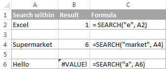
=SEARCH("market", "supermarket") returns 6 because the substring "market" begins at the 6th character of the word "supermarket".
=SEARCH("e", "Excel") returns 1 because "e" is the first character in the word "Excel", ignoring the case.
Like FIND, Excel's SEARCH function returns the #VALUE! error if:
- The value of the find_text argument is not found.
- The start_num argument is greater than the length of within_text.
- Start_num is equal to or less than zero.
Further on in this tutorial, you will find a few more meaningful formula examples that demonstrate how to use SEARCH function in Excel worksheets.
Excel FIND vs. Excel SEARCH
As already mentioned, the FIND and SEARCH functions in Excel are very much alike in terms of syntax and uses. However, they do have a couple of differences.
1. Case-sensitive FIND vs. case-insensitive SEARCH
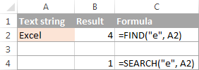
The most essential difference between the Excel SEARCH and FIND functions is that SEARCH is case-insensitive, while FIND is case-sensitive.
For example, SEARCH("e", "Excel") returns 1 because it ignores the case of "E", while FIND("e", "Excel") returns 4 because it minds the case.
2. Search with wildcard characters
Unlike FIND, the Excel SEARCH function accepts wildcard characters in the find_text argument:
- A question mark (?) matches one character, and
- An asterisk (*) matches any series of characters.
To see how it works on real data, consider the following example:
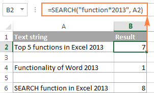
As you see in the screenshot above, the formula SEARCH("function*2013", A2) returns the position of the first character ("f") in the substring if the text string referred to in the within_text argument contains both "function" and "2013", no matter how many other characters there are in between.
Tip. To find an actual question mark (?) or asterisk (*), type a tilde (~) before the corresponding character.
Excel FIND and SEARCH formula examples
In practice, the Excel FIND and SEARCH functions are rarely used on their own. Typically, you would utilize them in combination with other functions such as MID, LEFT or RIGHT, and the following formula examples demonstrate some real-life uses.
Example 1. Find a string preceding or following a given character
This example shows how you can find and extract all characters in a text string to the left or to the right of a specific character. To make things easier to understand, consider the following example.
Supposing you have a column of names (column A) and you want to pull the First name and Last name into separate columns.
To get the first name, you can use FIND (or SEARCH) in conjunction with the LEFT function:
=LEFT(A2, FIND(" ", A2)-1)
or
=LEFT(A2, SEARCH(" ", A2)-1)
As you probably know, the Excel LEFT function returns the specified number of left-most characters in a string. And you use the FIND function to determine the position of a space (" ") to let the LEFT function know how many characters to extract. At that, you subtract 1 from the space's position because you don't want the returned value to include the space.
To extract the last name, use the combination of the RIGHT, FIND / SEARCH and LEN functions. The LEN function is needed to get the total number of characters in the string, from which you subtract the position of the space:
=RIGHT(A2,LEN(A2)-FIND(" ",A2))
or
=RIGHT(A2,LEN(A2)-SEARCH(" ",A2))
The following screenshot demonstrates the result:
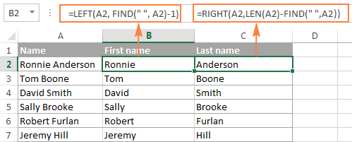
For more complex scenarios, such as extracting a middle name or splitting names with suffixes, please see How to split cells in Excel using formulas.
Example 2. Find Nth occurrence of a given character in a text string
Supposing you have some text strings in column A, say a list of SKUs, and you want to find the position of the 2nd dash in a string. The following formula works a treat:
=FIND("-", A2, FIND("-",A2)+1)
The first two arguments are easy to interpret: locate a dash ("-") in cell A2. In the third argument (start_num), you embed another FIND function that tells Excel to start searching beginning with the character that comes right after the first occurrence of dash (FIND("-",A2)+1).
To return the position of the 3rd occurrence, you embed the above formula in the start_num argument of another FIND function and add 2 to the returned value:
=FIND("-",A2, FIND("-", A2, FIND("-",A2)+1) +2)

Another and probably a simpler way of finding the Nth occurrence of a given character is using the Excel FIND function in combination with CHAR and SUBSTITUTE:
=FIND(CHAR(1),SUBSTITUTE(A2,"-",CHAR(1),3))
Where "-" is the character in question and "3" is the Nth occurrence you want to find.
In the above formula, the SUBSTITUTE function replaces the 3rd occurrence of dash ("-") with CHAR(1), which is the unprintable "Start of Heading" character in the ASCII system. Instead of CHAR(1) you can use any other unprintable character from 1 to 31. And then, the FIND function returns the position of that character in the text string. So, the general formula is as follows:
At first sight, it may seem that the above formulas have little practical value, but the next example will show how useful they are in solving real tasks.
Note. Please remember that the Excel FIND function is case-sensitive. In our example, this makes no difference, but if you are working with letters and you want a case-insensitive match, use the SEARCH function instead of FIND.
Example 3. Extract N characters following a certain character
To locate a substring of a given length within any text string, use Excel FIND or Excel SEARCH in combination with the MID function. The following example demonstrates how you can use such formulas in practice.
In our list of SKUs, supposing you want to find the first 3 characters following the first dash and pull them in another column.
If the group of characters preceding the first dash always contains the same number of items (e.g. 2 chars) this would be a trivial task. You could use the MID function to return 3 characters from a string, starting at position 4 (skipping the first 2 characters and a dash):
=MID(A2, 4, 3)
Translated into English, the formula says: "Look in cell A2, begin extracting from character 4, and return 3 characters".
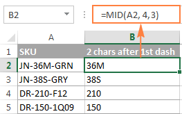
However, in real-life worksheets, the substring you need to extract could start anywhere within the text string. In our example, you may not know how many characters precede the first dash. To cope with this challenge, use the FIND function to determine the starting point of the substring that you want to retrieve.
The FIND formula to return the position of the 1st dash is as follows:
=FIND("-",A2)
Because you want to start with the character that follows the dash, add 1 to the returned value and embed the above function in the second argument (start_num) of the MID function:
=MID(A2, FIND("-",A2)+1, 3)
In this scenario, the Excel SEARCH function works equally well:
=MID(A2, SEARCH("-",A2)+1, 3)
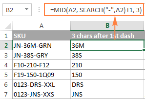
It's great, but what if the group of chars following the first dash contains a different number of characters? Hmm... this might be a problem:
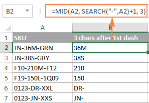
As you see in the above screenshot, the formula works perfectly for rows 1 and 2. In rows 4 and 5, the second group contains 4 characters, but only the first 3 chars are returned. In rows 6 and 7, there are only 2 characters in the second group, and therefore our Excel Search formula returns a dash following them.
If you wanted to return all chars between the 1st and 2nd occurrences of a certain character (dash in this example), how would you proceed? Here is the answer:
=MID(A2, FIND("-",A2)+1, FIND("-", A2, FIND("-",A2)+1) - FIND("-",A2)-1)
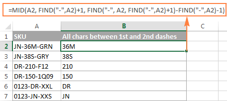
For better understanding of this MID formula, let's examine its arguments one by one:
- 1st argument (text). It's the text string containing the characters you want to extract, cell A2 in this example.
- 2nd argument (start_position). Specifies the position of the first character you want to extract. You use the FIND function to locate the first dash in the string and add 1 to that value because you want to start with the character that follows the dash: FIND("-",A2)+1.
- 3rd argument (num_chars). Specifies the number of characters you want to return. In our formula, this is the trickiest part. You use two FIND (or SEARCH) functions, one determines the position of the first dash: FIND("-",A2). And the other returns the position of the second dash: FIND("-", A2, FIND("-",A2)+1). Then you subtract the former from the latter, and then subtract 1 because you don't want to include either dash. As the result, you will get the number of characters between the 1st and 2nd dashes, which is exactly what we are looking for. So, you feed that value to the num_chars argument of the MID function.
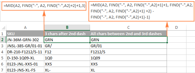
In a similar fashion, you can return 3 characters after the 2nd dash:
=MID(A2, FIND("-",A2, FIND("-", A2, FIND("-",A2)+1) +2), 3)
Or, extract all the characters between the 2nd and 3rd dashes:
=MID(A2, FIND("-", A2, FIND("-",A2)+1)+1, FIND("-",A2, FIND("-", A2, FIND("-",A2)+1) +2) - FIND("-", A2, FIND("-",A2)+1)-1)
Example 4. Find text between parentheses
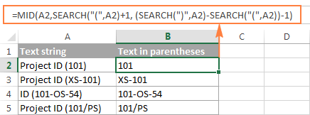
Supposing you have some long text string in column A and you want to find and extract only the text enclosed in (parentheses).
To do this, you would need the MID function to return the desired number of characters from a string, and either Excel FIND or SEARCH function to determine where to start and how many characters to extract.
=MID(A2,SEARCH("(",A2)+1, SEARCH(")",A2)-SEARCH("(",A2)-1)
The logic of this formula is similar to the ones we discussed in the previous example. And again, the most complex part is the last argument that tells the formula how many characters to return. That pretty long expression in the num_chars argument does the following:
- First, you find the position of the closing parenthesis:
SEARCH(")",A2) - After that you locate the position of the opening parenthesis:
SEARCH("(",A2) - And then, you calculate the difference between the positions of the closing and opening parentheses and subtract 1 from that number, because you don't want either parenthesis in the result:
SEARCH(")",A2)-SEARCH("(",A2))-1
Naturally, nothing prevents you from using the Excel FIND function instead of SEARCH, because case-sensitivity or case-insensitivity makes no difference in this example.
Hopefully, this tutorial has shed some light on how to use SEARCH and FIND functions in Excel. In the next tutorial, we are going to closely examine the REPLACE function, so please stay tuned. Thank you for reading!
 by
by
423 comments
Using VBA or other functions - how can i determine the position of a word or string in a drop down cell that has multiple values, then use that word or string position to find the corresponding number value in another cell with multiple values, so that I can sum up the quantity of the initial word or string?
For Example Cells A1:B2
A1 B1
Sprite 12
Coke 9
A2 B2
Rootbeer 3
Coke 21
So i want to sum the totals for Coke without having to split everything into single rows and columns?
Hi! Combine the values into a text string using the TEXTJOIN function. Then split these values into columns using the TEXTSPLIT function. Select the first column with the CHOOSECOLS function and compare it to the criterion.
Find the sum of matching values using the SUMPRODUCT function.
For example:
=SUMPRODUCT((CHOOSECOLS(TEXTSPLIT(TEXTJOIN(";",TRUE,A1:B2)," ",";"),1)="coke") * (CHOOSECOLS(TEXTSPLIT(TEXTJOIN(";",TRUE,A1:B2)," ",";"),2)))
Hello!
I wonder how to search for and return a text string from another sheet that can be sorted in different ways. Thats why I cant use a ordinary cell reference.
BR
Jörgen
Hello! If the words in a cell may be in a different order, you may need to search for a partial match. For more information, please read: How to find substring in Excel. There is not enough information for more detailed advice.
I have two excel columns. 1st column has a list of names. 2nd column has a description of the name and contain the name as well.
The two columns are not synced.
I want to extract the name from the 2nd column.
Tried using the function =SEARCH($A$1:$A$5,B1) as a part of my bigger function, but it's returning SPILL error and Value error.
Hi! You are doing a range search, so you get 5 results in your SEARCH calculation. This can cause a SPILL error, which you can read about in this article. Read about the VALUE error in the article above.
Thanks Alexander,
Looks like SEARCH is not the right function then for this. What would be a good formula to use for this task?
Hi! Based on your description, it is hard to completely understand your task. I don't know what you want to do. If you want to find a partial match of a text string in a range, use these instructions: How to find substring in Excel. To extract the corresponding value from another column, you can use this formula inside the INDEX MATCH function. For example:
=INDEX(C1:C10,MATCH(TRUE, ISNUMBER(SEARCH($A$1:$A$10,B1)),0))
Why do no articles explain what happens when NOT found, or how to deal with #VALUE?
I suggest you try searching. One article does explain your problem: #VALUE error in Excel: causes and fixes.
Hello and thank you very much for your excellent explanation.
I think the formula =FIND("-",A2, FIND("-", A2, FIND("-",A2)+1) +2) should be modified as follows.
=FIND("-",A2, FIND("-", A2, FIND("-",A2)+1) +1)
Hi Alex,
this is my first exposure to your forum and I'm impressed. Lots of clear, useful answers in a friendly tone. I actually found you while seeking a solution to the problem of getting #Value when the find_text is not found. I don't see an answer in the above, so here's what I came up with.
=IF(IFERROR(FIND("ZZ",$A$1),"No") "No",FIND("ZZ",$A$1),"Not found") /* Returns position of find_text start, or "Not Found" */
You probably have a better way of doing this, but I just wanted to add it as something that might be helpful to other searchers.
I see that the not equal symbols, meaning LessThan and GreaterThan, are missing from the above. I don't know if this is because I typed instead of copy/pasted or because this web interface swallowed them.
Anyway, there should be those two symbols between "No") and "No".
I'll try the copy/paste again:
=IF(IFERROR(FIND("ZZ",$A$1),"No")"No",FIND("ZZ",$A$1),"Not found")
Hi, I was hoping someone could please help me.
What is the best formula to archive the following;
1. Searching for the word car in cell AP1 i would like it to put the word DETAIL - this formula works
=IF(ISNUMBER(SEARCH("CAR",AP1)),"DETAIL",""
2. I also need the formula to search for the word "CLEAN" in addition to the word "CAR". How would i write this?
Below does not work.. What am I doing wrong?
=IF(ISNUMBER(SEARCH(or("CAR","CLEAN"),AP1)),"DETAIL",""
Hi! The SEARCH function can only search for one text string. Try this formula:
=IF(OR(ISNUMBER(SEARCH("CAR",A1)), ISNUMBER(SEARCH("CLEAN",A1))),"DETAIL","")
HELPFUL, THANKS
Hello,
I have a range of cells, AG2:AG100 with a string in each cell. There is a second list of string AA30:AA50 that I search if the string in this list is in the first list and return a third list ab30:ab50. The formula is in every cell AH2:AH100,
CELL AH2 formula is =IFERROR(INDEX($AB$30:$AB$44 & "", XMATCH(TRUE,ISNUMBER(IFERROR(SEARCH($AA$30:$AA$44,AG2), ""))),0),"")
With that advent of new functions like Lambda and BYROW I was wondering if you can accomplish the same task with only one formula in cell AH2 and spill down to ah100?
I have tried to nest BYROW function, but keep getting a #CALC error.
Thank you,
Hi! BYROW is a beta function currently only available through the Insiders channel in Excel 365
Hello Alexandar, Hope you're good, I want to use this function =IF(COUNTIF(B5:B10,"*"&D5&"*"), "YES","NO"), but instead of returning "YES" i need it to return the cell number (the one appears in name box) where my text was found.
Thanks in advance !!!
Hello! You can return the number of the cell in which a partial text match is found using the formula:
=MATCH(TRUE,ISNUMBER(SEARCH(D1,A:A)),0)
You can get the address of this cell using the ADDRESS function:
=ADDRESS(MATCH(TRUE,ISNUMBER(SEARCH(D1,A:A)),0),1,4)
How to determine if text strings are a partial match, read here: How to find substring in Excel.
Hello, Is there any way i can extract part of a string? I mean one without having any characters that divide them into smaller substrings like (; or -)
For example i have this text(RGSDAD00009VI5Y;5587172232783065), and i would like to get the middle 5 characters out, in this case 9VI5Y and nothing else. I mean without like actually counting them and using simple left right functions because there are a lot of them like this, and they aren't similar in length.
Thank you!
Hi! Explain what "middle 5 characters" means. There are 32 characters in your text, you want to extract from 11 to 15 characters.
Hi Alexander,
Really appreciate all the help you ae giving all of us! Much appreciated!
I am trying to extract a customer number from a column which contains text. The customer number always begins with the letter C and is exactly six digits in length - but we do not know what the numbers are bc they are for different customers transferring funds to us. The only thing we know is that the numbers can begin with only either 1 or 2. Sample customer numbers are: C202384, C219373, and also C198263, C154798. (Unfortunately there are other (non-important) words in the text which also have a C at the beginning but the following characters are all text and not numbers). I have looked all over the internet and find that there is no way to use this search pattern “C######” where # is an unknown number. If you are able to help that would be great. Also, if it is possible to continue with this theme and locate a six digit number within a cell containing text would also be very useful. This would be without an initial “C”. Thank, Alexander!
i.e.
Below is sample text which are contained in four cells.
Jellybean ltd C202748
Sq-219732 GEORGE, G
0000000
Received on:13JAN2023
DIRECT CREDIT
C202384 SP-219049 Brady Billott
0000000
Received on:13JAN2023
C104270 SP-219697
Keloo Barnyard
0000000
Received on:12JAN2023
RJHS 135
Cust 125655 ROBOCALL HIGH MESH
0000000
Received on:08JAN2023
Hi! To extract text by pattern, use regular expressions and the custom RegExpExtract function. You can find the examples and detailed instructions here: Regex to extract strings in Excel (one or all matches).
To extract the "C" and the 6 digits after it, try this formula:
=RegExpExtract(A1, "C\d{6}")
To extract the 6 digits after the space:
=TRIM(RegExpExtract(A1, " \d{6}"))
I recommend paying attention to the Regex tool. You can find, extract, compare, delete, or replace strings that match the regular expression pattern you enter. You don't need to install any VBA code. It is available as a part of our Ultimate Suite for Excel that you can install in a trial mode and check how it works for free.
I hope my advice will help you solve your task.
Hello Alexandar, Hope you're good, I wanted to join text from two columns for ex. In Cell A1 it is "Patient A + Patient B + Patient C" and in cell B1 some dose data is present ex. "240 mg, 1000 mg/m2, 100 mg/m2", now in C1, I want data to be like Patient A 240 mg + Patient B 1000 mg/m2 + Patient C 100 mg/m2, I want to do this in 1000 of rows, have tried Delimiting followed by CONTACT but not able to do the same for such big data, Could you pls help me out with a single formula in case possible, also what to do in case number increases for ex. In Cell A1 it is "Patient A + Patient B + Patient C + Patient D" and in cell B1 some dose data is present ex. "240 mg, 1000 mg/m2, 100 mg/m2, 10 mg", now in C1, I want data to be like Patient A 240 mg + Patient B 1000 mg/m2 + Patient C 100 mg/m2 + Patient D 10 mg.?
Hi! If I understand your task correctly, these articles may be helpful: TEXTJOIN function in Excel to merge text from multiple cells and TEXTSPLIT function in Excel: split text strings by delimiter. Try this formula:
=TEXTJOIN(" + ",TRUE,TEXTSPLIT(A1,,"+")&TEXTSPLIT(B1,,","))