These examples will teach you how to Vlookup multiple criteria, return a specific instance or all matches, do dynamic Vlookup in multiple sheets, and more.
It is the second part of the series that will help you harness the power of Excel VLOOKUP. The examples imply that you know how this function works. If not, it stands to reason to start with the basic uses of VLOOKUP in Excel.
Before moving further, let me briefly remind you the syntax:
Now that everyone is on the same page, let's take a closer look at the advanced VLOOKUP formula examples:
How to Vlookup multiple criteria
The Excel VLOOKUP function is really helpful when it comes to searching across a database for a certain value. However, it lacks an important feature - its syntax allows for just one lookup value. But what if you want to look up with several conditions? There are a few different solutions for you to choose from.
Formula 1. VLOOKUP with two criteria
Suppose you have a list of orders and want to find the quantity based on 2 criteria, Customer name and Product. A complicating factor is that each customer ordered multiple products, as shown in the table below:
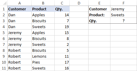
A usual VLOOKUP formula won't work in this situation because it returns the first found match based on a single lookup value that you specify.
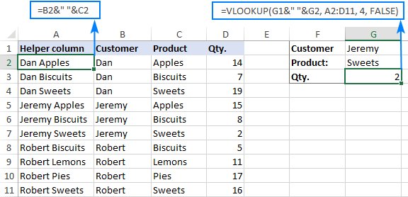
To overcome this, you can add a helper column and concatenate the values from two lookup columns (Customer and Product) there. It is important that the helper column should be the leftmost column in the table array because it's where Excel VLOOKUP always searches for the lookup value.
So, add a column to the left of your table and copy the below formula across that column. This will populate the helper column with the values from columns B and C (the space character is concatenated in between for better readability):
=B2&" "&C2
And then, use a standard VLOOKUP formula and place both criteria in the lookup_value argument, separated with a space:
=VLOOKUP("Jeremy Sweets", A2:D11, 4, FALSE)
Or, input the criteria in separate cells (G1 and G2 in our case) and concatenate those cells:
=VLOOKUP(G1&" "&G2, A2:D11, 4, FALSE)
As we want to return a value from column D, which is fourth in the table array, we use 4 for col_index_num. The range_lookup argument is set to FALSE to Vlookup an exact match. The screenshot below shows the result:
In case your lookup table is in another sheet, include the sheet's name in your VLOOKUP formula. For example:
=VLOOKUP(G1&" "&G2, Orders!A2:D11, 4, FALSE)
Alternatively, create a named range for the lookup table (say, Orders) to make the formula easier-to-read:
=VLOOKUP(G1&" "&G2, Orders, 4, FALSE)
For more information, please see How to Vlookup from another sheet in Excel.
Note. For the formula to work correctly, the values in the helper column should be concatenated exactly the same way as in the lookup_value argument. For example, we used a space character to separate the criteria in both the helper column (B2&" "&C2) and VLOOKUP formula (G1&" "&G2).
Formula 2. Excel VLOOKUP with multiple conditions
In theory, you can use the above approach to Vlookup more than two criteria. However, there are a couple of caveats. Firstly, a lookup value is limited to 255 characters, and secondly, the worksheet's design may not allow adding a helper column.
Luckily, Microsoft Excel often provides more than one way to do the same thing. To Vlookup multiple criteria, you can use either an INDEX MATCH combination or the XLOOKUP function recently introduced in Office 365.
For example, to look up based on 3 different values (Date, Customer name and Product), use one of the following formulas:
=INDEX(D2:D11, MATCH(1, (G1=A2:A11) * (G2=B2:B11) * (G3=C2:C11), 0))
=XLOOKUP(1, (G1=A2:A11) * (G2=B2:B11) * (G3=C2:C11), D2:D11)
Where:
- G1 is criteria 1 (date)
- G2 is criteria 2 (customer name)
- G3 is criteria 3 (product)
- A2:A11 is lookup range 1 (dates)
- B2:B11 is lookup range 2 (customer names)
- C2:C11 is lookup range 3 (products)
- D2:D11 is the return range (quantity)
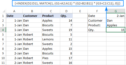
Note. In all versions except Excel 365, INDEX MATCH should be entered as an CSE array formula by pressing Ctrl + Shift + Enter. In Excel 365 that supports dynamic arrays it also works as a regular formula.
For the detailed explanation of the formulas, please see:
How to use VLOOKUP to get 2nd, 3rd or nth match
As you already know, Excel VLOOKUP can fetch only one matching value, more precisely, it returns the first found match. But what if there are several matches in your lookup array and you want to get the 2nd or 3rd instance? The task sounds quite intricate, but the solution does exist!
Formula 1. Vlookup Nth instance
Suppose you have customer names in one column, the products they purchased in another, and you are looking to find the 2nd or 3rd product bought by a given customer.
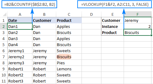
The simplest way is to add a helper column to the left of the table like we did in the first example. But this time, we will populate it with customer names and occurrence numbers like "John Doe1", "John Doe2", etc.
To get the occurrence, use the COUNTIF function with a mixed range reference (the first reference is absolute and the second is relative like $B$2:B2). Since the relative reference changes based on a position of the cell where the formula is copied, in row 3 it will become $B$2:B3, in row 4 - $B$2:B4, and so on.
Concatenated with the customer name (B2), the formula takes this form:
=B2&COUNTIF($B$2:B2, B2)
The above formula goes to A2, and then you copy it down to as many cells as needed.
After that, input the target name and occurrence number in separate cells (F1 and F2), and use the below formula to Vlookup a specific occurrence:
=VLOOKUP(F1&F2, A2:C11, 3, FALSE)
Formula 2. Vlookup 2nd occurrence
If you are looking for the 2nd instance of the lookup value, then you can do without the helper column. Instead, create the table array dynamically by using the INDIRECT function together with MATCH:
=VLOOKUP(E1, INDIRECT("A"&(MATCH(E1, A2:A11, 0)+2)&":B11"), 2, FALSE)
Where:
- E1 is the lookup value
- A2:A11 is the lookup range
- B11 is the last (bottom-right) cell of the lookup table
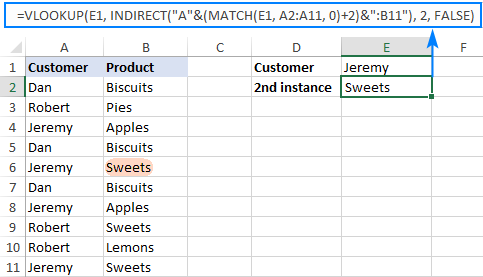
Please note that the above formula is written for a specific case where data cells in the lookup table begin in row 2. If your table is somewhere in the middle of the sheet, use this universal formula, where A1 is the top-left cell of the lookup table containing a column header:
=VLOOKUP(E1, INDIRECT("A"&(MATCH(E1, A2:A11, 0)+1+ROW(A1))&":B11"), 2, FALSE)
How this formula works
Here is the key part of the formula that creates a dynamic vlookup range:
INDIRECT("A"&(MATCH(E1, A2:A11, 0)+2)&":B11")
The MATCH function configured for exact match (0 in the last argument) compares the target name (E1) against the list of names (A2:A11) and returns the position of the first found match, which is 3 in our case. This number is going to be used as the starting row coordinate for the vlookup range, so we add 2 to it (+1 to exclude the first instance and +1 to exclude row 1 with the column headers). Alternatively, you can use 1+ROW(A1) to calculate the necessary adjustment automatically based on the position of the header row (A1 in our case).
As the result, we get the following text string, which INDIRECT converts to a range reference:
INDIRECT("A"&5&":B11") -> A5:B11
This range goes to the table_array argument of VLOOKUP forcing it to start searching in row 5, leaving out the first instance of the lookup value:
VLOOKUP(E1, A5:B11, 2, FALSE)
How to Vlookup and return multiple values in Excel
The Excel VLOOKUP function is designed to return just one match. Is there a way to Vlookup multiple instances? Yes, there is, though not an easy one. This requires a combined use of several functions such as INDEX, SMALL and ROW is an array formula.
For example, the below can find all occurrences of the lookup value F2 in the lookup range B2:B16 and return multiple matches from column C:
{=IFERROR(INDEX($C$2:$C$11, SMALL(IF($F$1=$B$2:$B$11, ROW($C$2:$C$11)-1,""), ROW()-1)),"")}
There are 2 ways to enter the formula in your worksheet:
- Type the formula in the first cell, press Ctrl + Shift + Enter, and then drag it down to a few more cells.
- Select several adjacent cells in a single column (F1:F11 in the screenshot below), type the formula and press Ctrl + Shift + Enter to complete it.
Either way, the number of cells in which you enter the formula should be equal to or larger than the maximum number of possible matches.
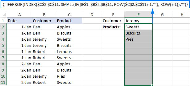
For the detailed explanation of the formula logic and more examples, please see How to VLOOKUP multiple values in Excel.
How to Vlookup in rows and columns (two-way lookup)
Two-way lookup (aka matrix lookup or 2-dimentional lookup) is a fancy word for looking up a value at the intersection of a certain row and column. There are a few different ways to do two-dimensional lookup in Excel, but since the focus of this tutorial is on the VLOOKUP function, we will naturally use it.
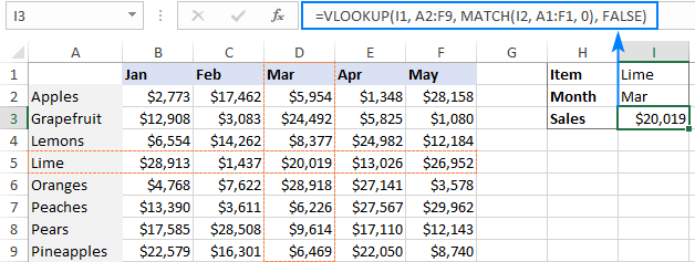
For this example, we'll take the below table with monthly sales and work out a VLOOKUP formula to retrieve the sales figure for a specific item in a given month.
With item names in A2:A9, month names in B1:F1, the target item in I1 and the target month in I2, the formula goes as follows:
=VLOOKUP(I1, A2:F9, MATCH(I2, A1:F1, 0), FALSE)
How this formula works
The core of the formula is the standard VLOOKUP function that searches for an exact match to the lookup value in I1. But since we do not know in which exactly column the sales for a specific month are, we cannot supply the column number directly to the col_index_num argument. To find that column, we use the following MATCH function:
MATCH(I2, A1:F1, 0)
Translated into English, the formula says: look up the I2 value in A1:F1 and return its relative position in the array. By supplying 0 to the 3rd argument, you instruct MATCH to find the value exactly equal to the lookup value (it's like using FALSE for the range_lookup argument of VLOOKUP).
Since Mar is in the 4th column in the lookup array, the MATCH function returns 4, which goes directly to the col_index_num argument of VLOOKUP:
VLOOKUP(I1, A2:F9, 4, FALSE)
Please pay attention that although the month names start in column B, we use A1:I1 for the lookup array. This is done in order for the number returned by MATCH to correspond to the column's position in table_array of VLOOKUP.
To learn more ways to perform matrix lookup in Excel, please see INDEX MATCH MATCH and other formulas for 2-dimensional lookup.
How to do multiple Vlookup in Excel (nested Vlookup)
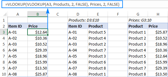
Sometimes it may happen that your main table and lookup table do not have a single column in common, which prevents you from doing a Vlookup between two tables. However, there exists another table, which does not contain the information you are looking for but has one common column with the main table and another common column with the lookup table.
In below image illustrates the situation:
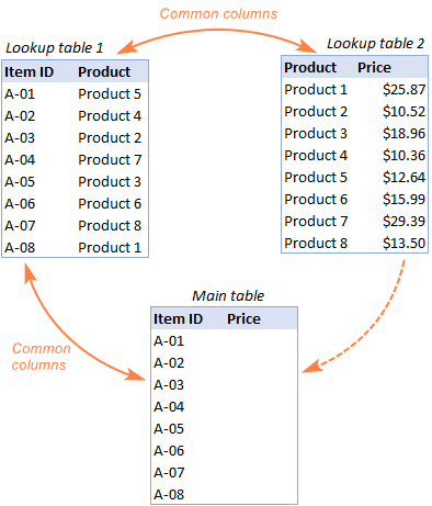
The goal is to copy prices to the main table based on Item IDs. The problem is that the table containing prices does not have the Item IDs, meaning we will have to do two Vlookups in one formula.
For the sake of convenience, let's create a couple of named ranges first:
- Lookup table 1 is named Products (D3:E10)
- Lookup table 2 is named Prices (G3:H10)
The tables can be in the same or different worksheets.
And now, we will perform the so-called double Vlookup, aka nested Vlookup.
First, make a VLOOKUP formula to find the product name in the Lookup table 1 (named Products) based on the item id (A3):
=VLOOKUP(A3, Products, 2, FALSE)
Next, put the above formula in the lookup_value argument of another VLOOKUP function to pull prices from Lookup table 2 (named Prices) based on the product name returned by the nested VLOOKUP:
=VLOOKUP(VLOOKUP(A3, Products, 2, FALSE), Prices, 2, FALSE)
The screenshot below shows our nested Vlookup formula in action:
How to Vlookup multiple sheets dynamically
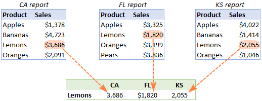
Sometimes, you may have data in the same format split over several worksheets. And your aim is to pull data from a specific sheet depending on the key value in a given cell.
This may be easier to understand from an example. Let's say, you have a few regional sales reports in the same format, and you are looking to get the sales figures for a specific product in certain regions:
Like in the previous example, we start with defining a few names:
- Range A2:B5 in CA sheet is named CA_Sales.
- Range A2:B5 in FL sheet is named FL_Sales.
- Range A2:B5 in KS sheet is named KS_Sales.
As you can see, all the named ranges have a common part (Sales) and unique parts (CA, FL, KS). Please be sure to name your ranges in a similar manner as it's essential for the formula we are going to build.
Formula 1. INDIRECT VLOOKUP to dynamically pull data from different sheets
If your task is to retrieve data from multiple sheets, a VLOOKUP INDIRECT formula is the best solution – compact and easy-to-understand.
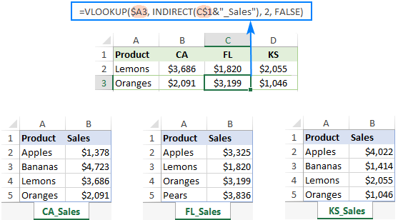
For this example, we organize the summary table in this way:
- Input the products of interest in A2 and A3. Those are our lookup values.
- Enter the unique parts of the named ranges in B1, C1 and D1.
And now, we concatenate the cell containing the unique part (B1) with the common part ("_Sales"), and feed the resulting string to INDIRECT:
INDIRECT(B$1&"_Sales")
The INDIRECT function transforms the string into a name that Excel can understand, and you put it in the table_array argument of VLOOKUP:
=VLOOKUP($A2, INDIRECT(B$1&"_Sales"), 2, FALSE)
The above formula goes to B2, and then you copy it down and to the right.
Please pay attention that, in the lookup value ($A2), we've locked the column coordinate with absolute cell reference so that the column remains fixed when the formula is copied to the right. In the B$1 reference, we locked the row because we want the column coordinate to change and supply an appropriate name part to INDIRECT depending on the column into which the formula is copied:
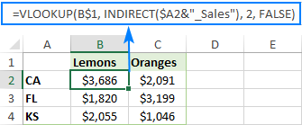
If your main table is organized differently, the lookup values in a row and unique parts of the range names in a column, then you should lock the row coordinate in the lookup value (B$1) and the column coordinate in the name parts ($A2):
=VLOOKUP(B$1, INDIRECT($A2&"_Sales"), 2, FALSE)
Formula 2. VLOOKUP and nested IFs to look up multiple sheets
In situation when you have just two or three lookup sheets, you can use a fairly simple VLOOKUP formula with nested IF functions to select the correct sheet based on the key value in a particular cell:
=VLOOKUP($A2, IF(B$1="CA", CA_Sales, IF(B$1="FL", FL_Sales, IF(B$1="KS", KS_Sales,""))), 2, FALSE)
Where $A2 is the lookup value (item name) and B$1 is the key value (state):

In this case, you do not necessarily need to define names and can use external references to refer to another sheet or workbook.
For more formula examples, please see How to VLOOKUP across multiple sheets in Excel.
That's how to use VLOOKUP in Excel. I thank you for reading and hope to see you on our blog next week!
Practice workbook for download
Advanced VLOOKUP formula examples (.xlsx file)
 by
by
521 comments
Thanks for this tutorial. You show how to find the VLOOKUP 2nd occurrence, but what would we change to find the 3rd, 4th or even 5th occurrence? I tried changing the +2 to +3, but my formula won't know exactly where the next occurrence is to know what row to start looking at. The 3rd occurrence could be on row 12 or 17 or not at all.
=VLOOKUP('Current Billing2'!AC2, INDIRECT("'Current Billing2'!AE"&(MATCH('Current Billing2'!AC2, 'Current Billing2'!AE2:AE17, 0)+2)&":AU7"), 14, FALSE)
Thanks!
Hi! I can't understand and check your formula as it contains unique references to data that I don't have.
Pay attention to the following paragraph of the article above: Vlookup and return nth match. In the formula
=VLOOKUP(F1&F2, A2:C11, 3, FALSE)
change the value of F2 to 3.
Thank you for responding and pointing me in the right direction! That specific idea didn't work for as I couldn't use a "helper column" however that lead me to find this solution:
=IF(IFERROR(VLOOKUP(SMALL(IF('Current Billing2'!AE2:AE11='Current Billing2'!AC2,ROW('Current Billing2'!AE2:AE11)),2),CHOOSE({1,2},ROW('Current Billing2'!AE2:AE11),'Current Billing2'!AR2:AR11),2,0),"")
Thanks again for the article!
I am using the VLOOKUP INDIRECT advice however when I plug in this formula in my desktop version
=VLOOKUP($A2, INDIRECT(B$1&"_Sales"), 2, FALSE)
my excel throws a #REF error
how do I correct this?
Thank you,
Hi! I don't know what kind of reference you were trying to get with the INDIRECT function, and I don't know what is written in cell B1.
If you wanted to get a reference to a named range, check what name is returned by B$1&"_Sales". For the detailed instructions, please see: How to use INDIRECT function in Excel - formula examples.
Your example of INDIRECT VLOOKUP seemed to have missed some parameter because as is, it gives me a "Volatile" result... once I add the reference column/rows then it works and brings me Oranges from CA_Sales. I just don't know why in your online excel version, your formula works but not when you do it in desktop version. Thank you
=VLOOKUP($A2, INDIRECT(B$1&"_Sales!A1:B5"), 2, FALSE)
Hi! You can download the sample file at the end of this article and see that all of these formulas work.
Amazing guide. thank you so much. this was a life saver.
I have two reports I need to combine, the first has a Customer ID, a Certificate # and an original balance (Column A, B , C respectively). The second report has the same info but balance spent, instead of original balance.
Each Customer ID has multiple Certificate #'s, and each Certificate # has multiple amounts for balance spent - Since VLOOKUP only matches the first line, I'm left with incomplete spend and remaining balance data.
I tried to use these formulas but couldn't figure out how to either combine the info first or get it to combine in the matching process.
Hi! Based on your description, it is hard to completely understand your task. I can assume that you want to calculate the amount of money spent on each of the certificate numbers. To do this, you can use the SUMIFS formula.
If you want to merge data from two tables using the Customer ID and Certificate # as the key columns, try to use the following guidelines: How to merge two or more tables in Excel.
If this does not help, explain the problem in more detail.
ORDER ID PRODUCT NAME CATEGORY NAME
10248 Queso Cabrales ??????
OrderID ProductID UnitPrice Quantity Discount
10248 11 14 12 0
ProductID ProductName SupplierID CategoryID QuantityPerUnit UnitPrice
1 Chai 1 1 10 boxes x 20 bags 18
CategoryID CategoryName Description
1 Beverages Soft drinks, coffees, teas, beers, and ales
The above are found in 4 different sheets. How do I use nested Vlookup to find the Category name. Note it has to be only vlookup. Please help
Your request goes beyond the advice we provide on this blog. This is a complex solution that cannot be found with a single formula. If you have a specific question about the operation of a function or formula, I will try to answer it. All the necessary information is in the article above.
How can you use this if there is a an "OR" for your criteria? Like if it can't find a name, it should look up a different column by phone number, and if there is a match with either it should return a specific column?
Hi! If I understand your question correctly, this article may be helpful: IF VLOOKUP in Excel: Vlookup formula with If condition.
Hi Alex,
I have a table which I am trying to format a function for. For context, It is for carbon footprint values of various products/materials. The table design is as below, and I am wondering if there is a way to use Vlookup in its current format.
column A - main category (e.g fuels, materials, waste.)
column B - sub category (in the case of fuels, e.g. solid, liquid, biofuel)
column C - sub-sub category (in the case of liquid fuel, e.g. diesel, petrol, gas oil, naphtha etc).
I currently have each item in column A merged into one cell, for example 'fuel' covers 48 rows. The single 'fuel' cell in column A spans 6 merged cells in column B (also covering 48 rows). One of these 6 is the 'liquid' section. The 'liquid' sub section of fuel contains 16 rows in column C. There are 48 items in column C each with their own row.
I currently have a 3 cell multi layered dependent drop down data validation formula set up.This allows the user to select an item from column A, e.g. Fuel (in cell P1). And then select an item from column B that is only within the fuel section, e.g liquid (in cell Q1). Finally selecting an item from column C only within the liquid section under fuels (in cell R1).
My issue, is that throughout the table I have multiple repeats of wordings in column C I may not be able to get around. I am currently using a Vlookup formula based on the drop down selection from column C (cell R1). This unfortunately only picks up the first iteration of the wording in column C over the whole table (circa 900 rows).
How can I edit the vlookup formula to factor in the results from column A and B?
If you shoot me an email I'd be happy to run through the document with you on a call.
Kind regards,
Jack
Hi! The VLOOKUP or INDEX MATCH formula extracts only the first record from the table that matches the search criteria. To get all matches at once, you can try the FILTER function. Read more: Excel FILTER function - dynamic filtering with formulas.
How can I get VLOOKUP to do this?
Column A has many values, some of them duplicates. Not all of the duplicates have a value in column B.
When i enter a new value in cell A1000 (Mike) i want to have a formula in cell B1000 like this:
=VLOOKUP(A1000, $A$1:$B999,2,0) but if the value is blank then keep searching until you find the next "Mike" column A that does have a value in its corresponding B cell.
in the case below I'd like to return a value of "ALIEN"
Row # Column A Column B
1 Mike (blank)
2 John cat
3 Anna dog
4 Beatrice man
5 Mike
6 Terry bird
7 Francis worm
8 Mike ALIEN
1000 (New entry (formula here to find the first non-blank cell in column B for Mike)
named) Mike
Hi! You can find the desired non-empty value using the INDEX MATCH function. Based on your information, the formula might look something like this:
=INDEX($B$1:B999,MATCH(1,($A$1:A999=A1000)*($B$1:B999<>""),0))
You can find the examples and detailed instructions here: Excel INDEX MATCH with multiple criteria - formula examples
figured it out:
=IFERROR(INDEX($B$2:$B999,MATCH(1,IF($A$2:$A999=A1000,IF($B$2:$B999"",1)),0)),"")
I have a downloaded report from a website that has a lot of merged cells and not in a vlookup friendly format. Is there a formula that will do a dual lookup. Lookup this name and bring in a lookup for this row this column #? I know there are some new lookup formulas, I just can find the right one.
Example: I would need a formula that searches for the Name of Business, and lookup up the row and add the # column to pull. I would probably need to do a row range also.
Name of Business
2021 2022 2023
Cost
Sales
Profit
Hi! Based on your description, it is hard to completely understand your task. However, I’ll try to guess and pay attention to this section in the article above: How to Vlookup in rows and columns (two-way lookup), as well as this article: INDEX MATCH MATCH in Excel for two-dimensional lookup. If this does not help, explain the problem in detail.
I need to pull pricing data based off quantity amount using wither the VLOOKUP or IF functions, I'm not sure. Lets see if I can make sense of this.
Column A: part numbers, Column B: web price, Column C: Quantities, Column D: web price based off quantity purchased. So the pricing is based off scale, meaning thew more you buy, the the cheaper the product. How do I create a VLOOKUP function that will pull the part number pricing based on quantity purchased?
Hi! To find the price by two criteria (part numbers, quantity) read carefully the paragraph in the article above: How to Vlookup multiple criteria. You can also find useful information in this article: Excel INDEX MATCH with multiple criteria - formula examples.
What I have wrong? I need to look for Assigned and Work in progress words in one excel column
=IFERROR(VLOOKUP(A2 & ="Assigned"),FULL!A:U,9,0),N2) + (A2& ="Work in progress"),FULL!A:U,9,0),N2)
Hi! From your description, it is difficult to have a full understanding of your task. However, I’ll try to guess and offer you the following formula:
=IFERROR(VLOOKUP("Assigned",A:U,14,0),IFERROR(VLOOKUP("Work in progress",A:U,14,0),""))
You can also find useful information in this article: VLOOKUP with IF statement in Excel.
i have patient data list in from column A to D ( example Colum A, MR No, Colum B, Name, Colom C, Medicine, Colom D, Labs, C etc)
I need your help How to VLOOKUP and return multiple values when I enter the MR no in cell and get others information from colm b to c
Hello! You can create a separate VLOOKUP formula in each of the columns of B, and so on, to get the value you want for the MR criterion. All the information you need to do this is in the article above.
You can use the FILTER function to apply a filter to your table as described in this guide: Excel FILTER function - dynamic filtering with formulas.
Hello,
I have a difficulty to use any formula, for a very simple task. I always get an error like #VALUE or #N/A as result and I do not understand why.
In Table 1 , there is in C2 the PlantName W01 and in A44 is the Process Name = Casting, and I want to get from Table 2 the corresponding ScrapCost matching to these 2 values in the Table 1, in the D44 Cell. I used VLOOKUP, INDEX/MATCH, and I always get an error and I do not know why?
The Table 2 has several Columns with O4:O157 = PlantNames , from Q1:Q25 ProcessesNames (repeating for each plant until Cell Q157), and corresponding ScrapCost is in T4 :T157 (for each PlantName and each ProcessName).
Can you help me ?
Hi! I’m sorry but your description doesn’t give me a complete understanding of your task. Correct me if I’m wrong, but I believe the formula below will help:
=INDEX(T4:T157,MATCH(1,(O4:O157=C2)*(Q4:Q157=A44),0))
I recommend reading this guide: Excel INDEX MATCH with multiple criteria - formula examples.
Hello I Have Data Like One Lookup But Different Cells Example One Sheet Lookup Attendence And The Data Different Cells Like Colum Number 2,3,4,5,6,7,8,9,10 So How Can Lookup One Click Atten.But Same At Is Work For Drage
Hi! Unfortunately, this information is not enough to understand what you need.
Hi I need to add a price against multiple duplicate part numbers, the Vlookup function works so far, then the formula goes wrong as the column index number starts to run sequentially. example below. So the Vlookup works and it's pulling across the cost correctly. But there are 30 duplicate part numbers following this one, and this is where vlookup goes wrong. rather than looking at the same cell from the sheet 1 data for each duplicate it starts to look at the cell below, so doesn't return a correct value.
Branch Part Qty Picked Cost
AYRE AGLBTG325 1 1 £4.99
=VLOOKUP(B367,Sheet1!A56:B515,2,0)
Sheet 1 Data
Part Cost
AGLBTG325 4.99
Branch Part Qty Picked Cost
AYRE AGLBTG325 1 1 £4.99
BIRS AGLBTG325 1 1 #N/A
Vlookup formula for next duplicate down
=VLOOKUP(B368,Sheet1!A369:B516,2,0)
As you can see it's looking sequentially on sheet1 rather than looking at cell A56, so the next cell down is now looking at A370. How do i get it to stop doing that? Any help would be appreciated as there's 149 part numbers but a total of 1474 duplicates I need to cost up.
Hi! I’m not sure, I got you right, since the description you provided is not entirely clear. Maybe this article will be helpful: How to copy formula in Excel with or without changing references. For example:
=VLOOKUP(B367,Sheet1!$A$56:$B$515,2,0)
If this is not what you wanted, please describe the problem in more detail.
Hi. I am trying to do a VLOOKUP that searches for multiple lookup values. For example, I know this syntax doesn't exist, but I want to achieve something like this =VLOOKUP(H4 OR H5, A1:B10,2,). My return values in this case are all numbers, so ideally I'd like it to look for any values matching cells H4 or H5, then sum all corresponding values and return. In this case there may be a value only in H4, only in H5, or both. Is this possible??
Hi! To sum values by condition, use the SUMIF function. For example:
=SUMIF(A1:A20,H4,B1:B20)+SUMIF(A1:A20,H5,B1:B20)
Also, to find the sum by multiple criteria, try the SUMPRODUCT function:
=SUMPRODUCT(((A1:A20=H4)+(A1:A20=H5))*B1:B20)
Hi, I would like to ask for a formula for a scenario below:
If enter a Name in B2, output will be as below:
B2: Name
B3: Address
B4: Age
B5: Contact Number
B6: Email Address
B7: School
thank you for the help
Hi! You can get all the values in cells B3:B7 using the VLOOKUP or INDEX MATCH formula. I can't recommend an exact formula to you, as I can't see your data.
Hi, i am trying to use vlookup get 2 results within one request - e.g If the data if found within the array then the resulting cell is to be multiplied by a specific cell, but if the data is NOT found then the resulting cell should be multiplied by a different cell
=VLOOKUP(A1,$B$1:$B$5,1,0)*$C$1 - works if the condition is true (the match is found) - but how do i include the same equation withen the formula if the condition isnt true (the match isn't found) - which i would them want it to be then multiplied by a different cell e.g $c$2
Hi! I don't really understand what you want to multiply if no value is found. To display some value instead of an error message, use the IFERROR function. For example:
= IFERROR (VLOOKUP(A1,$B$1:$B$5,1,0)*$C$1,C2)
OMG. I had a huge list of people that had different "interests" and "expertise". Each category (interest and expertise) had about 15 subcategories that people could select from. In querying my database I could easily pull a list of people, but the data returned had a separate row for each person/category/subcategory. Not uncommon for a database query.
But, I was preparing data for a mail-merge, so I needed to create a file that had each individual person listed on a single row. Then I needed to create columns for each category/subcategory pairing. Getting the names for the mail-merge was easy; I could just pull the name from the database dump, paste into a new sheet, and then remove duplicates. But figuring out how to match the info in the category/subcategory columns was crazy hard since there needed to be 3 things that matched: Name, Category, Subcategory.
The XLOOKUP option worked perfectly. Still not exactly sure what all the items are (like why we use "1" as the lookup_value) and the Office 365 sort features were slightly different than what was used here. But between the great explanation here combined with the prompts in Excel for the last few items, made it workable. Then it was just cut/paste formulas into various columns and tweak the category/subcategory options for each cat/subcat column.
Thank you so so sooooooooo much.
Sample for clarification:
Converting from - (I added the Return Value column to my database dump for insertion into the modified mail-merge table)
Individual Category Subcategory Return Value
Person X Category 1 Subcategory 1 X
Person X Category 2 Subcategory 1 X
Person X Category 2 Subcategory 2 X
Person Y Category 1 Subcategory 1 X
Person Y Category 2 Subcategory 1 X
Person Z Category 1 Subcategory 2 X
Person Z Category 2 Subcategory 1 X
Into - (for mail-merge purposes)
Individual Category 1/Subcategory 1 Category 1/Subcategory 2 Category 2/Subcategory 1 Category 2/Subcategory 2
Person X X X X
Person Y X X
Person Z X X
LOL. Okay, the "extra" spaces to try and make it look table-like didn't come through, but hopefully you get the idea. And everything did work swimmingly.
Hi! Unfortunately, your request goes beyond the advice we provide on this blog. This is a complex solution that cannot be found with a single formula. If you have a specific question about the operation of a function or formula, I will try to answer it.
I have a worksheet with different file numbers for the same account
Account number is in column A and file numbers in B
Please give me a formula where it will give me all the multiple values in column B for an account number in column A
Thank you
Hi! Look for the example formulas here: How to Vlookup multiple values in Excel with criteria.
please tell me the formula for different columns data to lookup for same values . for ex : order id AB022365 , column heading 1 order status( delivered/undelivered , colun2 (complaint), column 3( branch)and so on . but formula must work together .
Hi! Based on your description, it is hard to completely understand your task. However, I’ll try to guess and offer you the following guide: How to highlight duplicate cells and rows in Excel. If this does not help, explain the problem in detail.
Hello, I am looking for formula where I have a row on product with multiple information in columns. I have to base information from two column and return back value from column 1. For example:
Houses Cars Office
Matt 3 2 2
Venkat 4 1 3
Lars 2 3 6
Sam 8 4 5
Output I want to know person with 2 houses and 1 car
I want to know person with 3 houses and 4 cars
How can this be done?
Hi! If I understand your task correctly, you can find the examples and detailed instructions here:: Excel INDEX MATCH with multiple criteria. The formula might look like this:
=INDEX(A1:A10,MATCH(1,(B1:B10=2)*(C1:C10=1),0))
I'm looking for a formula that will look up a date in column A, then lookup a name in column C, then look up a category from row 1, and return the value when all three has been met.
I have tried using the following =INDEX(AU2:DJ139,MATCH(C2,AU2:AU5000)*(B21,AW2:AW5000)*(F20,AU1:DJ1),0) but get #N/A returned.
Any suggestions as to what formula will look up all three and return the value would appreciated.
Hi! To do a multi-criteria search, look for the example formulas here: Excel INDEX MATCH with multiple criteria.
Also note that all ranges in the formula must be the same size.
I hope I answered your question. If something is still unclear, please feel free to ask.
Good afternoon,
I am unable to find a formula to produce a correct value in a spreadsheet. I have two worksheets (DR and PI).
DR contains complete records and PI contains the records I am reviewing. I need excel to find PI cell value of A9 and PI cell value of I9 in a single row in the DR raw data, and when those values match return the value of DR column 11 to PI.
Hi! To search for two values, use the INDEX MATCH functions. However, your information is not enough to give you more accurate advice. In which cells will you search for these values? To understand what you want to do, give an example of the source data and the expected result.
I am using the VLOOKUP function to search for values in one workbook (Workbook 2 cells: F513 = 515,600.05 and cell F518 = 96,560.46) 6 columns to the right of column A, based on multiple values in another workbook, within ONE cell (Workbook 1 cell A15 = 401-05-0000, 403-01-0000. I would like the results to be added together and the result placed in one cell (Workbook 1 cell G15. How should I modify the VLOOKUP function below at the red arrow to do this?
=VLOOKUP(A15,'[BVAR Balanza julio 2023.xlsx]Balanza de Comprobación'!$A$387:$F$834,6,FALSE)
Thank you
David
Sorry, ignore "at the red arrow to do this?". I could not post a screen shot. I just want to know how to modify the VLOOKUP to accomplish the above.
Thank you,
David
Hi! To sum multiple values based on several criteria, try using the SUMIFS function. Read more: Excel SUMIFS and SUMIF with multiple criteria – formula examples.
How many sources of importrange i can use for vlookup?
I am not sure I fully understand what you mean.
HI I have two sheets.
Sheet 1 is where i want to see the result (Allocated time) and Sheet 2 is the source. There are two criteria to look at 1 is the country 2 is the service provider 1-5. Main goal is to catch the number of hours assign for each service provider in a given country.
Sheet 1
Belgium Provider 1 Allocated Time based on Sheet 2
Belgium Provider 2 Allocated Time based on Sheet 2
Belgium Provider 3 Allocated Time based on Sheet 2
Belgium Provider 4 Allocated Time based on Sheet 2
Belgium Provider 5 Allocated Time based on Sheet 2
In the source sheet 2, you'll notice that the provider is not in sequence like in Sheet 1
Sheet 2
Belgium Provider 3 Allocated time
Belgium Provider 5 Allocated time
Belgium Provider 2 Allocated time
Belgium Provider 1 Allocated time
Belgium Provider 4 Allocated time
Hi,
I have a query how to vlookup on multiple conditions.
my data
I have emp id in column A, emp details in Colom D and values in column E
my qurey is I want to vlookup for column A 1st and match with column D and get the results of E in to my results cell.
column D have multiple rows like basic pay, DA, HRA etc column A have emp id
here is the sample data
1010408 RAMESH RUPIREDDY Personnel#: 1010408 BASIC PAY 1,85,430.00
1010408 RAMESH RUPIREDDY Name: RAMESH RUPIREDDY Basic GPF Arr 7,57,185.00
1010408 RAMESH RUPIREDDY Desig ADE STAGNATION PAY 12,240.00
1010408 RAMESH RUPIREDDY Seat No: CPRS-S2-1 Stagnation Pay GPF -52,860.00
1010408 RAMESH RUPIREDDY BANK: SBHY0020138 Stagnation Pay EPF 69,779.00
1010408 RAMESH RUPIREDDY A/c No 52135288942 D.A. 11,655.00
1010408 RAMESH RUPIREDDY Net Pay: 181559 D A(GPF) Arr -4,17,824.00
1010408 RAMESH RUPIREDDY PPO No D A(EPF) Arr 2,391.00
1010408 RAMESH RUPIREDDY H.R.A 21,000.00
1010408 RAMESH RUPIREDDY HRA Arr 78,001.00
Request to provide the me formula for this
Hi! Unfortunately, this information is not enough to understand what you need. Specify what results you want in column E for each row of your data sample. Describe your task in more detail.
my day is like this
Personnel#: 1010408 BASIC PAY 1,27,185.00 GIS -120
Name: RAMESH RUPIREDDY STAGNATION PAY 4,405.00 GPF Contribution -8,000.00
Desig ADE Stagnation Pay GPF 17,620.00 DA Cr to GPF 4,370.00
Seat No: CPRS-S2-1 D.A. 37,685.00 LIC -5,074.00
BANK: SBHY0020138 D A(GPF) Arr 4,726.00 Professional Tax -200
A/c No 52135288942 H.R.A 15,000.00 INCOME TAX -50,000.00
Net Pay: 135743 GENERATION ALLOWAN 24,637.00 SFMS -500
PPO No COAL HANDLING ALLO 455 bank loan -36,650.00
CONVEYANCE ALLOWAN 1,500.00 society -5,170.00
Shift Allw 6,822.00
Sl.No 2 Leave encashment A 2 Total Deductions -1,10,084.00
CUG ALLOWANCE 83
PLF ALLOWANCE 2,767.00
TELANGANA INCREMEN 955
24X7 POWER INCREME 1,985.00
Earnings 25,115.00
Earnings 2,20,712.00
Total Earnings 2,45,827.00
************ ***************************** ****************** ********************************** ********************** *****************
Personnel#: 1010410 BASIC PAY 1,31,590.00 GIS -360
Name: SANTOSH PASPULATTI Basic GPF Arr 3,46,520.00 GPF Contribution -7,895.00
Desig ADE D.A. 37,685.00 DA Cr to GPF 17,428.00
Seat No: CPRS-S2-1 D A(GPF) Arr 96,198.00 LIC -27,822.00
BANK: SBHY0020138 H.R.A 15,000.00 Professional Tax -600
A/c No 52135320498 HRA Arr 43,500.00 INCOME TAX -1,96,300.00
Net Pay: 474143 GENERATION ALLOWAN 24,637.00 SFMS -1,500.00
PPO No Gen.Allw Arr 6,358.00
COAL HANDLING ALLO 455 Total Deductions -2,51,905.00
Coal Handling Allo 117
Sl.No 3 CONVEYANCE ALLOWAN 1,500.00
Conveyance Allw Ar 387
Shift Allw 6,822.00
Shift Allw Arr 1,761.00
CUG ALLOWANCE 83
CUG Allowance Arr 83
PLF ALLOWANCE 1,598.00
TELANGANA INCREMEN 955
TELANGANA INCREMEN 2,515.00
24X7 POWER INCREME 2,280.00
24X7 POWER INCREME 6,004.00
Earnings 5,05,041.00
Earnings 2,21,007.00
Total Earnings 7,26,048.00
************ ***************************** ****************** ********************************** ********************** *****************
Personnel#: 1010411 BASIC PAY 1,35,995.00 GIS -120
Name: RAMESH BANDI F.P.I 75 GPF Contribution -20,000.00
Desig ADE D.A. 38,946.00 LIC -6,125.00
Seat No: CPRS-S2-1 GENERATION ALLOWAN 24,637.00 Professional Tax -200
BANK: SBHY0020138 Gen.Allw Arr -367 INCOME TAX -37,100.00
A/c No 52135294116 COAL HANDLING ALLO 455 SFMS -500
Net Pay: 138147 Shift Allw Arr -1,320.00
PPO No PLF ALLOWANCE 536 Total Deductions -64,045.00
TELANGANA INCREMEN 955
24X7 POWER INCREME 2,280.00
Sl.No 4
Earnings -1,151.00
Earnings 2,03,343.00
Total Earnings 2,02,192.00
************ ***************************** ****************** ********************************** ********************** *****************
Personnel#: 1035357 BASIC PAY 2,48,330.00 GIS -120
Name: SURESH KUMAR ERIKI STAGNATION PAY 10,560.00 GPF Contribution -15,533.00
Desig ADE F.P.I 860 LIC -3,154.00
Seat No: CPRS-S2-1 D.A. 74,141.00 Professional Tax -200
BANK: SBIN0021031 H.R.A 15,000.00 INCOME TAX -99,600.00
A/c No 52108831007 GENERATION ALLOWAN 24,637.00 SFMS -500
Net Pay: 270998 DUST ALLOWANCE 275
PPO No CONVEYANCE ALLOWAN 1,500.00 Total Deductions -1,19,107.00
Shift Allw 6,822.00
CUG ALLOWANCE 83
Sl.No 5 PLF ALLOWANCE 2,767.00
TELANGANA INCREMEN 1,750.00
24X7 POWER INCREME 3,380.00
Earnings 2,767.00
Earnings 3,87,338.00
Total Earnings 3,90,105.00
what I want is I want get all these into a table format
like
Sno Personnel#: BASIC PAY STAGNATION PAY F.P.I D.A. GENERATION ALLOWAN COAL HANDLING ALLO CONVEYANCE ALLOWAN Shift Allw CUG ALLOWANCE PLF ALLOWANCE TELANGANA INCREMEN 24X7 POWER INCREME Total Earnings GSLISA GIS GPF Contribution Professional Tax INCOME TAX CC CHARGES CC CHARGES SFMS Total Deductions
the raw data is consist of 100's of employees
I want the data transposed to table format with above headers and corresponding values, each employee data is separated with ******* row and for each emp have the earning in one column and deduction in another column
really appreciated your help
thank you in advance.
is there a way to share the sample file let me know so it will be much easier to understand
I want formula for two sheet vlookup then i want c column value against b& a
Hi! Look for the example formulas here: How to VLOOKUP across multiple sheets in Excel with examples.
? I have sheet for real estate customer payment for rent each customer with deferent code number have how can i make the formula for each code that remind me to pay then the status for each customer after unpaid show paid on that date.
please support me
Please clarify your specific problem or provide additional details to highlight exactly what you need. As it's currently written, it's hard to tell exactly what you're asking.
WELL STRING TEST DATE BLPD
A 01/01/2015 1,246
B 05/10/2018 879
C 07/03/2015 1,135
D 12/09/2015 674
A 06/10/2015 978
B 28/12/2015 0
C 20/01/2015 1,498
D 02/07/2015 957
A 10/08/2015 1,189
B 15/11/2015 654
C 21/05/2015 1,359
D 31/01/2015 31
.....Continue
This is the data i have. In this data the well string name is going to repeat multiple times with different test date & BLPD value.
Now i have another set of data as follows:
WELL STRING ACTIVITY DATE TEST DATE NEAREST TO ACTIVITY DATE BLPD
A 04/02/2015 ? ?
B 07/11/2018 ? ?
C 12/04/2015 ? ?
D 13/08/2015 ? ?
A 05/12/2015 ? ?
B 26/11/2015 ? ?
C 10/03/2015 ? ?
D 04/08/2015 ? ?
A 12/07/2015 ? ?
B 14/10/2015 ? ?
C 25/06/2015 ? ?
D 31/07/2015 ? ?
How to enter the formula for question mark?
Sorry, I do not fully understand the task. To understand what you want, give examples of the desired result.
For example: In 1st row of second data base... Well String A has activity date 04/02/2015. In row 1 Column C3 of database 2, we want "TEST DATE NEAREST TO ACTIVITY DATE". Now we go to data base 1 & search the test date nearest to activity date 4/02/2015 for Well String A. In database 1, we can see there are 3 test dates against well string A & the test date nearest to activity date(04/02/2015) is 01/01/2015. So in database 2: R1C3 will be 01/01/2015 & R1C4( BLPD: Barrel Liquid per day) will be 1,246 as given in database1. I want Column 3 & Column 4 of database 2 to be derived from database 1 with the help of formula. Please suggest.
Hello! Use the FILTER function to get values for Well String A only. Then use INDEX MATCH function to find the BLPD value for the nearest date.
=INDEX(FILTER('1'!A1:C12,'1'!A1:A12='2'!A1), MATCH(MIN(ABS('2'!B1-FILTER('1'!B1:B12,'1'!A1:A12='2'!A1))), ABS('2'!B1-FILTER('1'!B1:B12,'1'!A1:A12='2'!A1)),0),3)
Hope this is what you need.