In our previous tutorial, we were looking at Excel If contains formulas that return some value to another column if a target cell contains a given value. Aside from that, what else can you do if a cell contains specific text or number? A variety of things such as counting or summing cells, highlighting, removing or copying entire rows, and more.
Excel 'Count if cell contains' formula examples
In Microsoft Excel, there are two functions to count cells based on their values, COUNTIF and COUNTIFS. These functions cover most, though not all, scenarios. The below examples will teach you how to choose an appropriate Count if cell contains formula for your particular task.
Count if cell contains any text
In situations when you want to count cells containing any text, use the asterisk wildcard character as the criteria in your COUNTIF formula:
Or, use the SUMPRODUCT function in combination with ISTEXT:
In the second formula, the ISTEXT function evaluates each cell in the specified range and returns an array of TRUE (text) and FALSE (not text) values; the double unary operator (--) coerces TRUE and FALSE into 1's and 0's; and SUMPRODUCT adds up the numbers.
As shown in the screenshot below, both formulas yield the same result:
=COUNTIF(A2:A10,"*")
=SUMPRODUCT(--(ISTEXT(A2:A10)))
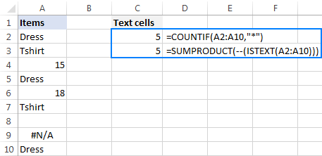
You may also want to look at how to count non-empty cells in Excel.
Count if cell contains specific text
To count cells that contain specific text, use a simple COUNTIF formula like shown below, where range is the cells to check and text is the text string to search for or a reference to the cell containing the text string.
For example, to count cells in the range A2:A10 that contain the word "dress", use this formula:
=COUNTIF(A2:A10, "dress")
Or the one shown in the screenshot:
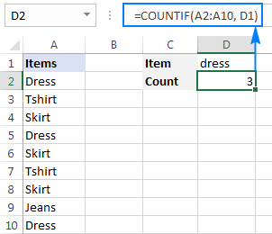
You can find more formulas examples here: How to count cells with text in Excel: any, specific, filtered cells.
Count if cell contains text (partial match)
To count cells that contain a certain substring, use the COUNTIF function with the asterisk wildcard character (*).
For example, to count how many cells in column A contain "dress" as part of their contents, use this formula:
=COUNTIF(A2:A10,"*dress*")
Or, type the desired text in some cell and concatenate that cell with the wildcard characters:
=COUNTIF(A2:A10,"*"&D1&"*")
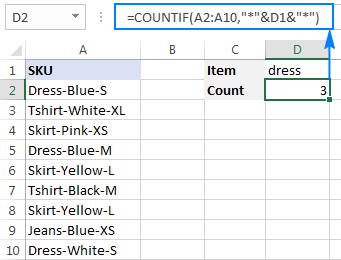
For more information, please see: COUNTIF formulas with partial match.
Count if cell contains multiple substrings (AND logic)
To count cells with multiple conditions, use the COUNTIFS function. Excel COUNTIFS can handle up to 127 range/criteria pairs, and only cells that meet all of the specified conditions will be counted.
For example, to find out how many cells in column A contain "dress" AND "blue", use one of the following formulas:
=COUNTIFS(A2:A10,"*dress*", A2:A10,"*blue*")
Or
=COUNTIFS(A2:A10,"*"&D1&"*", A2:A10,"*"&D2&"*")
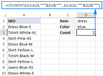
Count if cell contains number
The formula to count cells with numbers is the simplest formula one could imagine:
Please keep in mind that the COUNT function in Excel counts cells containing any numeric value including numbers, dates and times, because in terms of Excel the last two are also numbers.
In our case, the formula goes as follows:
=COUNT(A2:A10)
To count cells that DO NOT contain numbers, use the SUMPRODUCT function together with ISNUMBER and NOT:
=SUMPRODUCT(--NOT(ISNUMBER(A2:A10)))
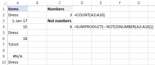
For more examples, see Excel formulas to count cells with certain text.
Sum if cell contains text
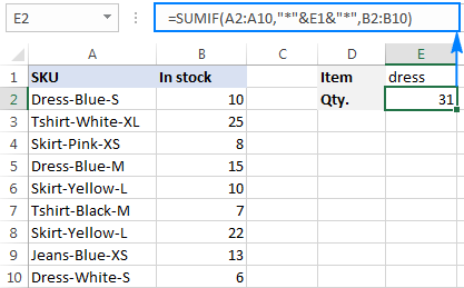
If you are looking for an Excel formula to find cells containing specific text and sum the corresponding values in another column, use the SUMIF function.
For example, to find out how many dresses are in stock, use this formula:
=SUMIF(A2:A10,"*dress*",B2:B10)
Where A2:A10 are the text values to check and B2:B10 are the numbers to sum.
Or, put the substring of interest in some cell (E1), and reference that cell in your formula, as shown in the screenshot below:
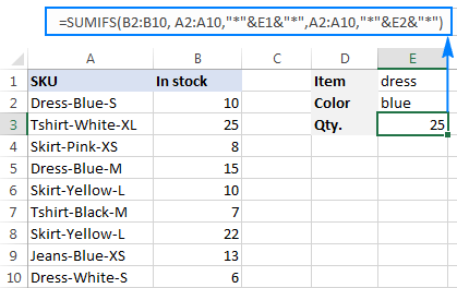
To sum with multiple criteria, use the SUMIFS function.
For instance, to find out how many blue dresses are available, go with this formula:
=SUMIFS(B2:B10, A2:A10,"*dress*",A2:A10,"*blue*")
Or use this one:
=SUMIFS(B2:B10, A2:A10,"*"&E1&"*",A2:A10,"*"&E2&"*")
Where A2:A10 are the cells to check and B2:B10 are the cells to sum.
Perform different calculations based on cell value
In our last tutorial, we discussed three different formulas to test multiple conditions and return different values depending on the results of those tests. And now, let's see how you can perform different calculations depending on the value in a target cell.
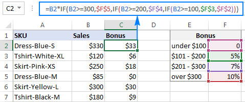
Supposing you have sales numbers in column B and want to calculate bonuses based on those numbers: if a sale is over $300, the bonus is 10%; for sales between $201 and $300 the bonus is 7%; for sales between $101 and $200 the bonus is 5%, and no bonus for under $100 sales.
To have it done, simply multiply the sales (B2) by a corresponding percentage. How do you know which percentage to multiply by? By testing different conditions with nested IFs:
=B2*IF(B2>=300,10%, IF(B2>=200,7%, IF(B2>=100,5%,0)))
In real-life worksheets, it may be more convenient to input percentages in separate cells and reference those cells in your formula:
=B2*IF(B2>=300,$F$5,IF(B2>=200,$F$4,IF(B2>=100,$F$3,$F$2)))
The key thing is fixing the bonus cells' references with the $ sign to prevent them from changing when you copy the formula down the column.
Excel conditional formatting if cell contains specific text
If you want to highlight cells with certain text, set up an Excel conditional formatting rule based on one of the following formulas.
Case-insensitive:
Case-sensitive:
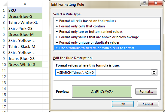
For example, to highlight SKUs that contain the words "dress", make a conditional formatting rule with the below formula and apply it to as many cells in column A as you need beginning with cell A2:
=SEARCH("dress", A2)>0
Excel conditional formatting formula: if cell contains text (multiple conditions)
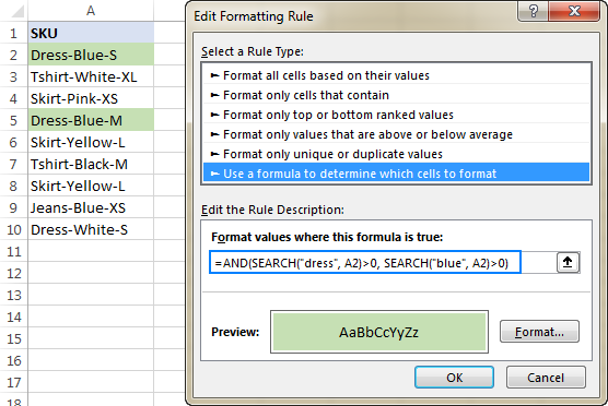
To highlight cells that contain two or more text strings, nest several Search functions within an AND formula. For example, to highlight "blue dress" cells, create a rule based on this formula:
=AND(SEARCH("dress", A2)>0, SEARCH("blue", A2)>0)
For the detailed steps, please see How to create a conditional formatting rule with a formula.
If cell contains certain text, remove entire row
In case you want to delete rows containing specific text, use Excel's Find and Replace feature in this way:
- Select all cells you want to check.
- Press Ctrl + F to open the Find and Replace dialog box.
- In the Find what box, type the text or number you are looking for, and click the Find All
- Click on any search result, and then press Ctrl + A to select all.
- Click the Close button to close the Find and Replace
- Press Ctrl and the minus button at the same time (Ctrl -), which is the Excel shortcut for Delete.
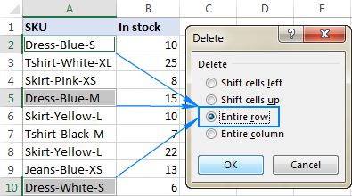
- In the Delete dialog box, select Entire row, and click OK. Done!
In the screenshot below, we are deleting rows containing "dress":
If cell contains, select or copy entire rows
In situations when you want to select or copy rows with relevant data, use Excel's AutoFilter to filter such rows. After that, press Ctrl + A to select the filtered data, Ctrl+C to copy it, and Ctrl+V to paste the data to another location.
To filter cells with two or more criteria, use Advanced Filter to find such cells, and then copy the entire rows with the results or extract only specific columns.
This is how you manipulate cells based on their value in Excel. I thank you for reading and hope to see you on our blog next week!
Practice workbook
Excel If Cell Contains Then - examples (.xlsx file)
 by
by
236 comments
I tried using SUBTOTAL(Function,Range to count). Excel provides you an option to Select the operation (Add/Subtract/Divide etc..) under Function and range of values where you need to count and list in another cell. My requirement was to Sum the value in a range based on filter selected.
Hi! The answer to your question can be found in this article: Excel SUBTOTAL function with formula examples.
Argument Function 101 - 111 ignore all hidden cells - filtered out and hidden manually. For example:
=SUBTOTAL(109,C2:C20)
I have a spreadsheet with quotes, quote amount, PO and then finaly invoice number. I want to calculate on the lines that has a inv number on the quote amount. In other words what has been invoiced.
Hi! To find the total amount for a specific invoice number, you can use the COUNTIF function. If you need to find a sum for more than one condition, use these instructions: How to use Excel COUNTIFS and COUNTIF with multiple criteria.
Hi,
I have a sheet of our business with various branches in our region. I pull a report daily from our ERP system of all the products with stock codes starting with "F" i.e. "Fxxxxxxx"
The branch name is in column A, the Stock codes are in Column B and the sales value of each product is in column E.
I need a formula to extract the total sales value for each branch on stock items with F codes. Can anyone help?
Hi! You can use the SUMIF formula to determine the value of sales for a specific branch. Read more: How to use SUMIF function in Excel with formula examples. Use these instructions if you have multiple conditions to summarize: Excel SUMIFS and SUMIF with multiple criteria. I hope it’ll be helpful. If something is still unclear, please feel free to ask.
using this formula
=SUMIFS(C1:C5,A1:A5,D1,B1:B5,D2)
if my DATA is this
Chocolate || _____ || 4 |Chocolate
Brown Sugar || 1kg || 3 || ______
if my data for D1 is chocolate why it will show "0" but if my Data in D1 is Brown Sugar 1kg it will count? what is my error?
Hi! The SUMIFS formula cannot use an empty cell as a criterion. If 0 is written in the cell, the formula will work.
My sheet contains drop down lists. Cell C5 has 4 options and Cells D7:M7 have 3. I need a formula that will add D9:M9 if Cell C5 contains "Summit", or "ARTC", or "Empower" AND if D7:M7 contains "SL 1:1". I have been trying to figure out how to do this for 2 days now and would really appreciate some help.
Hi! If I understand your task correctly, this guide may be helpful: Nested IF with OR/AND conditions.
I can't offer you an example formula, as I don't understand what "formula that will add D9:M9" and "D7:M7 contains "SL 1:1"" mean. But I think that with the help of these instructions you will be able to solve the problem.