The tutorial shows how to use ISBLANK and other functions to identify blank cells in Excel and take different actions depending on whether a cell is empty or not.
There are many situations when you need to check if a cell is empty or not. For instance, if cell is blank, then you might want to sum, count, copy a value from another cell, or do nothing. In these scenarios, ISBLANK is the right function to use, sometimes alone, but most often in combination with other Excel functions.
Excel ISBLANK function
The ISBLANK function in Excel checks whether a cell is blank or not. Like other IS functions, it always returns a Boolean value as the result: TRUE if a cell is empty and FALSE if a cell is not empty.
The syntax of ISBLANK assumes just one argument:
Where value is a reference to the cell you want to test.
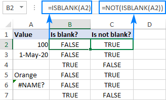
For example, to find out if cell A2 is empty, use this formula:
=ISBLANK(A2)
To check if A2 is not empty, use ISBLANK together with the NOT function, which returns the reversed logical value, i.e. TRUE for non-blanks and FALSE for blanks.
=NOT(ISBLANK(A2))
Copy the formulas down to a few more cells and you will get this result:
ISBLANK in Excel - things to remember
The main point you should keep in mind is that the Excel ISBLANK function identifies truly empty cells, i.e. cells that contain absolutely nothing: no spaces, no tabs, no carriage returns, nothing that only appears blank in a view.
For a cell that looks blank, but in fact is not, an ISBLANK formula returns FALSE. This behavior occurs if a cell contains any of the following:
- Formula that returns an empty string like IF(A1<>"", A1, "").
- Zero-length string imported from an external database or resulted from a copy/paste operation.
- Spaces, apostrophes, non-breaking spaces ( ), linefeed or other non-printing characters.

How to use ISBLANK in Excel
To gain more understanding of what the ISBLANK function is capable of, let's take a look at some practical examples.
Excel formula: if cell is blank then
Since Microsoft Excel does not have a built-in IFBLANK kind of function, you need to use IF and ISBLANK together to test a cell and perform an action if the cell is empty.
Here's the generic version:
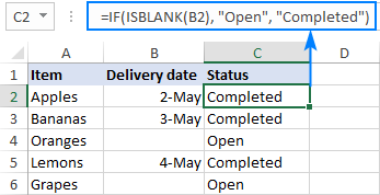
To see it in action, let's check if a cell in column B (delivery date) has any value in it. If the cell is blank, then output "Open"; if the cell is not blank, then output "Completed".
=IF(ISBLANK(B2), "Open", "Completed")
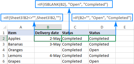
Please remember that the ISBLANK function only determines absolutely blank cells. If a cell contains something invisible to the human eye such as a zero-length string, ISBLANK would return FALSE. To illustrate this, please have a look at the screenshot below. The dates in column B are pulled from another sheet with this formula:
=IF(Sheet3!B2<>"",Sheet3!B2,"")
As the result, B4 and B6 contain empty strings (""). For these cells, our IF ISBLANK formula yields "Completed" because in terms of ISBLANK the cells are not empty.
If your classification of "blanks" includes cells containing a formula that results in an empty string, then use ="" for the logical test:
=IF(B2="", "Open", "Completed")
The screenshot below shows the difference:
Excel formula: if cell is not blank then
If you've closely followed the previous example and understood the formula's logic, you should have no difficulties with modifying it for a specific case when an action shall only be taken when the cell is not empty.
Based on your definition of "blanks", choose one of the following approaches.
To identify only truly non-blank cells, reverse the logical value returned by ISBLANK by wrapping it into NOT:
Or use the already familiar IF ISBLANK formula (please notice that compared to the previous one, the value_if_true and value_if_false values are swapped):
To teat zero-length strings as blanks, use <>"" for the logical test of IF:
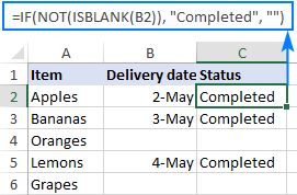
For our sample table, any of the below formulas will work a treat. They all will return "Completed" in column C if a cell in column B is not empty:
=IF(NOT(ISBLANK(B2)), "Completed", "")
=IF(ISBLANK(B2), "", "Completed")
=IF(B2<>"", "Completed", "")
If cell is blank, then leave blank
In certain scenarios, you may need a formula of this kind: If cell is blank do nothing, otherwise take some action. In fact, it's nothing else but a variation of the generic IF ISBLANK formula discussed above, in which you supply an empty string ("") for the value_if_true argument and the desired value/formula/expression for value_if_false.
For absolutely blank cells:
To regard empty strings as blanks:
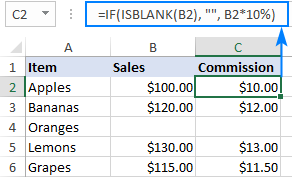
In the table below, suppose you want to do the following:
- If column B is empty, leave column C empty.
- If column B contains a sales number, calculate the 10% commission.
To have it done, we multiply the amount in B2 by percentage and put the expression in the third argument of IF:
=IF(ISBLANK(B2), "", B2*10%)
Or
=IF(B2="", "", B2*10%)
After copying the formula through column C, the result looks as follows:
If any cell in range is blank, then do something
In Microsoft Excel, there are a few different ways to check a range for empty cells. We will be using an IF statement to output one value if there is at least one empty cell in the range and another value if there are no empty cells at all. In the logical test, we calculate the total number of empty cells in the range, and then check if the count is greater than zero. This can be done with either COUNTBLANK or COUNTIF function:
Or a little bit more complex SUMPRODUCT formula:
For example, to assign the "Open" status to any project that has one or more blanks in columns B through D, you can use any of the below formulas:
=IF(COUNTBLANK(B2:D2)>0,"Open", "")
=IF(COUNTIF(B2:D2,"")>0, "Open", "")
=IF(SUMPRODUCT(--(B2:D2=""))>0, "Open", "")
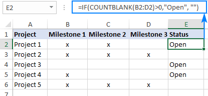
Note. All these formulas treat empty strings as blanks.
If all cells in range are blank, then do something
To check if all cells in the range are empty, we will be using the same approach as in the above example. The difference is in the logical test of IF. This time, we count cells that are not empty. If the result is greater than zero (i.e. the logical test evaluates to TRUE), we know that not every cell in the range is blank. If the logical test is FALSE, that means all cells in the range are blank. So, we supply the desired value/expression/formula in the 3rd argument of IF (value_if_false).
In this example, we will return "Not Started" for projects that have blanks for all the milestones in columns B through D.
The easiest way to count non-empty cells in Excel is by using the COUNTA function:
=IF(COUNTA(B2:D2)>0, "", "Not Started")
Another way is COUNTIF for non-blanks ("<>" as the criteria):
=IF(COUNTIF(B2:D2,"<>")>0, "", "Not Started")
Or the SUMPRODUCT function with the same logic:
=IF(SUMPRODUCT(--(B2:D2<>""))>0, "", "Not Started")
ISBLANK can also be used, but only as an array formula, which should be completed by pressing Ctrl + Shift + Enter, and in combination with the AND function. AND is needed for the logical test to evaluate to TRUE only when the result of ISBLANK for each cell is TRUE.
=IF(AND(ISBLANK(B2:D2)), "Not Started", "")
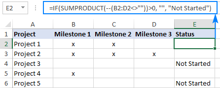
Note. When choosing a formula for your worksheet, an important thing to consider is your understanding of "blanks". The formulas based on ISBLANK, COUNTA and COUNTIF with "<>" as the criteria look for absolutely empty cells. SUMPRODUCT also regards empty strings as blanks.
Excel formula: if cell is not blank, then sum
To sum certain cells when other cells are not blank, use the SUMIF function, which is especially designed for conditional sum.
In the table below, supposing you wish to find the total amount for the items that are already delivered and those that are not yet delivered.
If not blank then sum
To get the total of delivered items, check if the Delivery date in column B is not blank and if it isn't, then sum the value in column C:
=SUMIF(B2:B6, "<>", C2:C6)
If blank then sum
To get the total of undelivered items, sum if the Delivery date in column B is blank:
=SUMIF(B2:B6, "", C2:C6)

Sum if all cells in range are not blank
To sum cells or perform some other calculation only when all cells in a given range are not blank, you can again use the IF function with the appropriate logical test.
For example, COUNTBLANK can bring us the total number of blanks in the range B2:B6. If the count is zero, we run the SUM formula; otherwise do nothing:
=IF(COUNTBLANK(B2:B6)=0, SUM(B2:B6), "")
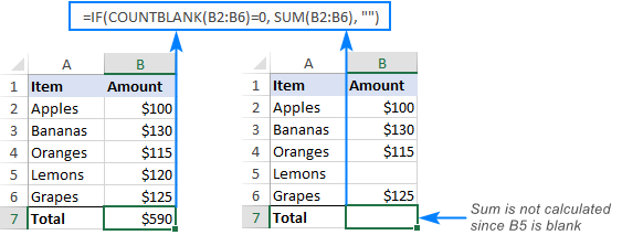
The same result can be achieved with an array IF ISBLANK SUM formula (please remember to press Ctrl + Shift + Enter to complete it correctly):
=IF(OR(ISBLANK(B2:B6)), "", SUM(B2:B6))
In this case, we use ISBLANK in combination with the OR function, so the logical test is TRUE if there is at least one blank cell in the range. Consequently, the SUM function goes to the value_if_false argument.
Excel formula: count if cell is not blank
As you probably know, Excel has a special function to count non-empty cells, the COUNTA function. Please be aware that the function counts cells containing any type of data, including the logical values of TRUE and FALSE, error, spaces, empty strings, etc.
For example, to count non-blank cells in the range B2:B6, this is the formula to use:
=COUNTA(B2:B6)
The same result can be achieved by using COUNTIF with the non-blank criteria ("<>"):
=COUNTIF(B2:B6,"<>")
To count blank cells, use the COUNTBLANK function:
=COUNTBLANK(B2:B6)

Excel ISBLANK not working
As already mentioned, ISBLANK in Excel returns TRUE only for really empty cells that contain absolutely nothing. For seemingly blank cells containing formulas that produce empty strings, spaces, apostrophes, non-printing characters, and the like, ISBLANK returns FALSE.
In a situation, when you want to treat visually empty cells as blanks, consider the following workarounds.
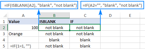
Treat zero-length strings as blanks
To consider cells with zero-length strings as blanks, in the logical test of IF, put either an empty string ("") or the LEN function equal to zero.
=IF(A2="", "blank", "not blank")
Or
=IF(LEN(A2)=0, "blank", "not blank")
Remove or ignore extra spaces
In case the ISBLANK function is malfunctioning because of blank spaces, the most obvious solution is to get rid of them. The following tutorial explains how to quickly remove leading, trailing and multiple in-between spaces, except for a single space character between words: How to remove extra spaces in Excel.
If for some reason removing excess spaces does not work for you, you can force Excel to ignore them.
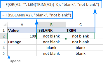
To regard cells containing only space characters as empty, include LEN(TRIM(cell))=0 in the logical test of IF as an additional condition:
=IF(OR(A2="", LEN(TRIM(A2))=0), "blank", "not blank")
To ignore a specific non-printing character, find its code and supply it to the CHAR function.
For example, to identify cells containing empty strings and nonbreaking spaces ( ) as blanks, use the following formula, where 160 is the character code for a nonbreaking space:
=IF(OR(A2="", A2=CHAR(160)), "blank", "not blank")
That's how to use the ISBLANK function to identify blank cells in Excel. I thank you for reading and hope to see you on our blog next week!
 by
by
50 comments
Is there any formula for this:
If A is blank it will show B
Please re-check the article above since it covers your task.
i would be grateful if anyone can help with the below query.
as i keep filling the column list , a specific cell keeps updating as per the filled next cell and if not then shows as per the last updated column list.
Hello!
I have a situation where three cells have formulas. I need a formula that calculates four different ways, as follows:
if(and a2="X",b2=""c2="" - then h2*$U$13
if(and b2>0,a2=""c2="" - then h2*$U$12
if(and c2="X",a2=""b2="" - then h2*$U$15
if a2:c2="",h2*$U$11
This formula returns only blank -
=IF(SUMPRODUCT(--(a2:c2""))>0,SUM(H2*$U$11),IF(a2="x",SUM(h2*$U$13),IF(c2="X",SUM(h2*$U$15),"")))
This formula returns only the result of h2*u11 -
=IF(OR(COUNTBLANK(a2:c2)>0),H2*$U$11,IF(AND(a2="x",ISBLANK(b2)=""),H2*$U$13,IF(AND(b2="x",ISBLANK(c2)=""),H2*$U$15)))
This following formulas only return the result of h2*u12 -
=IF(D2="x",H2*$U$13,IF(ISBLANK(E2)>0,H2*$U$12,IF(F2="x",H2*$U$15,IF(COUNTBLANK(D2:F2)>0,H2*$U$11,))))
=IF(COUNTBLANK(a2:c2)>0,H2*$U$11,IF(AND(a2="x",ISBLANK(b2)="",ISBLANK(c2)=""),H2*$U$13,IF(AND(c2="x",ISBLANK(a2)="",ISBLANK(b2)=""),H2*$U$15,IF(AND(b2>0,ISBLANK(a2)="",ISBLANK(c2)=""),H2*$U$12))))
I have tried every formula I can think of and nothing is producing an "as expected" result. I have spent a great deal of time on this and al at a total loss.
I would be eternally grateful for any help you could provide! Thank you!
Hi! If I got you right, the formula below will help you with your task:
=IFS(AND(A2="X",B2="",C2=""), H2*$U$13, AND(B2>0,A2="",C2=""), H2*$U$12, AND(C2="X",A2="",B2=""), H2*$U$15, AND(C2="",A2="",B2=""), H2*$U$11)
Look for the example formulas here: Excel IFS function instead of multiple IF.
If i have a materials due back within 10 days of issuance, but nothing has come back (so cell is blank) how do i calculate the days overdue?
the formula i've used so far is
=IF(F18>=G18,(G18-F18),(Today()-G18)) <-- but once cell G18 has a date it will continue to count days using (TODAY()-G18) but i would like it to stop counting after materials are received.
Task:
Worksheet with 3 tabs
Each tab has multiple columns and rows of data
I want unique values from column 2 where they = "CD" and column 9 is not zero
I've created this equation:
"=TOCOL(SORT(UNIQUE(CHOOSECOLS(LET(CDCOM,VSTACK(Ours!$B$4:$J$100,CAD!$B$4:$J$100,DAD!$B$4:$J$100),FILTER(CDCOM,(INDEX(CDCOM,,2)="CD"))),1))))"
I can't figure out how Excel will allow me to add in the second criteria. I checked whether column 2 was "CD" and that worked. Then I got back a row that had no values, ie zero in column 9. I need to check whether column 2 = "CD" and column 9 is not zero. I tried MATCH after index with 2 criteria but it fails? I'm either missing the issue, or Excel won't let me add a second criteria, doesn't sound right, but.......
Thanks for your time
David
PS - Keep up the good work, I've become a follower for Excel information from you guys, very easy to read and follow, excellent job!
Hi! It is very difficult to understand a formula that contains unique references to your workbook worksheets. I can't check a formula that contains unique references to your data, which I don't have. Please clarify your specific problem or provide additional information to understand what you need.
I am trying to create a condition whereby I have a summary sheet and it is linked to another sheet with '√' and 'X' and I keyed-in a formula to return blank for the portions that are blank that are linked. But the problem comes when I want to return blank on the formulated cells which returned a blank from the previous sheet.
Eg, Sheet 1 Sheet 2
Clmn Clmn 1 Clmn 2
Row Row
1 √ =if(isblank(sheet1A1),"",sheet1A1) =if(isblank(A1),"",if(A1="√),"PASS","FAIL")
2 √ =if(isblank(sheet1A2),"",sheet1A2)
3 X =if(isblank(sheet1A3),"",sheet1A3)
4
5
Is there any work around on this? I want the empty cells (with formula) to return blank in Column 2. Thanks in advance
Hello!
The cell where the formula is written is not empty. Try using A1="" instead of ISBLANK(A1)
1 coloum A coloum B coloum c
03/02/23 05/02/23 =today()-a answer 1
2 blank blank =?
i want to know this how we put formula here to count the days
=today()-a1 how to use this formula to count days if have blank cell
Hi!
To calculate by condition, use the IF function
=IF(ISBLANK(A1),"",TODAY()-A1)
Hope this is what you need.
i using this formula to count for days =today()-a1
but if i have blank cell then how we count the days.
Dear Sir,
kindly help me this kinda data
if the data is
Sr.no Yash Sumit Sujay Rahul R
1. 5. 3.
2. 1. 6
In Sr.no 1
if Sumit and Rahul data is blank then the result will be headings of the blank cell in the end column (R)
i.e Sumit,Rahul
and result for Sr.no 2 = Yash,Sujay
Hi!
Sorry, it's not quite clear what you are trying to achieve.
Hi Alexander
I couldn't believe that you replied so quickly, as I only finished & pushed sent when I got your reply, (how quick is the internet) but thank you very much as this taken about 2 years of searching & I did find other information.
So with the formula I did change -3 & +3 to -1 & +1 for MID also -6 & +5 for LEFT to get the results that I was looking for.
11.06 (4)
=IF(ISBLANK(A268),"",MID(A268,SEARCH("(",A268)+1,SEARCH(")",A268)-SEARCH("(",A268)-1)) Result 4
=IF(ISBLANK(A268),"",MID(A268,SEARCH("(",A268)-6,SEARCH(")",A268)-SEARCH("(",A268)+4)) Result 11.06
Thank You
Regards
Tont
Hi Alexander
Is there a way to use a both formula's below & isblank in the same formula's?
11.06 (4) =MID(A268,FIND("(",A268)+1,FIND(")",A268)-FIND("(",A268)-1) Result 4
=LEFT(A268,SEARCH("(",A268)-1) Result 11.06
10.83 (-) =MID(A269,FIND("(",A269)+1,FIND(")",A269)-FIND("(",A269)-1) Result -
=LEFT(A269,SEARCH("(",A269)-1) Result 10.83
The one with (-) Result is to return blank?
The other question is can ISBLANK FORMULA WORK ON A ISBLANK FORMULA & return blank?
Any help or direction would be greatly appreciated
Regards
Tony
Hi Alexander
Is it possible to use ISBLANK with MID function from (0:12.41) & formula below
=MID(B375,SEARCH("(",B375)+3,SEARCH(")",B375)-SEARCH("(",B375)-3)
to return 12.41 or blank ?
Regards
Tony
Hello!
If I understand you correctly, you want to check if the cell is empty. To do this, you can use the ISBLANK function
=IF(ISBLANK(B375),"",MID(B375,SEARCH("(",B375)+3,SEARCH(")",B375)-SEARCH("(",B375)-3))
Thank you for reading this. Is it possible to order the cells after using 'isblank'?
I currently have:
Date Rank
05/05/2022 1
06/05/2022 2
04/05/2022 3
01/05/2022 4
Blank cells indicate no data, because of 'isbank'! Ideally, I'd have the Rank in date order.
Hi!
I’m sorry but your description doesn’t give me a complete understanding of your task. Correct me if I’m wrong, but I believe the formula below will help:
=RANK.EQ(A1,$A$1:$A$10,1)
You can copy this formula down along the column.
You can learn more about RANK.EQ function in Excel in this article on our blog.
Thank you - here's more of the chart:
Colour Date Rank
Red 05/05/2022 1
Green
Blue 06/05/2022 2
Black
Yellow
Purple 01/05/2022 3
Orange
Lilac 03/05/2022 4
Where would I put the Rank formula you kindly posted, to enable me to see the colours in date order?
Hi!
If you want to sort column A by non-empty cells in column B, then use the FILTER and SORT functions:
=SORT(FILTER(A1:B10,NOT(ISBLANK(B1:B10))),2,-1)
Hope this is what you need.
Hello,
I am creating a list of parts and if a part is on list one but not on list two I want excel to automatically add the part to the blank at the end of list one. I am stuck on this one and cant think of any way to do this with a formula. Do you have any ideas?
Thank you
I have a nested IF formula that I want to add another parameter too but I am stuck as follows -
If Cell L2 is blank, I need the number of days between column A and today but if L2 has a date, I calculate the number of days between A2 and L2. This is fine using the formula below which uses networkdays to ignore certain dates:
=IF(ISBLANK(L2),NETWORKDAYS(A2,Today(),Lists!$G$2:$G$49974),NETWORKDAYS(L2,Today(),Lists!$G$2:$G$49974))
What I am trying to do in addition to the above is to say that if Cell R2 has a date in it, to ignore the formula above and to count the days between A2 and R2.
Just to complicate things, I also have S2 with a date (but R2 and S2 will not both be populated, only one or the other), so the formula needs to include that if R2 or S2 have a date, then calculate the days between A2 and R2 or A2 and S2 but if both are blank, then keep the numbers in the above formula.
I have tried many permutations formulas but without success and I would be grateful for your advice.
Sorry if this is confusing.
Thanks
Hello!
Please have a look at this article - Excel Nested IF statement: examples, best practices and alternatives
=IF(ISBLANK(S2),IF(ISBLANK(R2),IF(ISBLANK(L2), NETWORKDAYS(A2,TODAY(),$G$2:$G$49974), NETWORKDAYS(L2,TODAY(),$G$2:$G$49974)), NETWORKDAYS(R2,TODAY(),$G$2:$G$49974)), NETWORKDAYS(S2,TODAY(),$G$2:$G$49974))
Many thanks for your quick reply Alexander. I had to amend your suggestion as the $G2:$G$49974 referred to a list of days on a separate sheet called Lists, but once I added that bit back, it worked a dream. Many thanks again for a speedy and time saving reply.
Hi, I am trying to use this "double" formula to check two sets of criteria:
1. range a5:q5 = one criteria (checks if all the cells in this criteria are blank)
2. second range (smaller) = another criteria (checks if only some of the cells in this criteria are blank)
Formula is:
=IF(SUMPRODUCT(--(a5:q5""))>0,"","No ref and ax", IF(SUMPRODUCT(--(k5:q5""))>0,"","T2 ax not complete"))
I have also tried using IF(OR( and IF(AND( but I have a similar issue.
Both formulas work separately, but not together.
Hello!
Multiple conditions can be combined using the CHOOSE function:
=CHOOSE(IF(SUMPRODUCT(--(A5:Q5 < > ""))>0,0,1)+ IF(SUMPRODUCT(--(K5:Q5 < > ""))>0,0,2)+1,"", "No ref and ax","T2 ax not complete", "No ref and ax"&" T2 ax not complete")
I hope I answered your question. If you have any other questions, please don’t hesitate to ask.
Thanks Alexander! This worked a treat :)
Thank you for taking the time to reply.
this is my formula i am using.
=IF(ISBLANK(B11)*ISBLANK(C11),"",SUM(D10+B11-C11))
so i am counting my pto hours. i have a column for "accured" (B column) and "taken" (C column). then i have a 3rd column(D) which is the amount of pto i have. when i have blanks in the cells in the B and C columns then my Cell in the D column is blank unless i fill in the cells. so example:
B3 is blank and C3 is blank so D3 will be blank. What i want it to do is if both B and C cells are blank then show the value in D2 cell. so if D2 cell shows 20 and B3 and C3 are blank then show D2 value of 20 in D3 cell. but if B3 and C3 are filled in then do the sum function.
Hi!
I am not sure I fully understand what you mean.
The formula cannot set the values of 2 cells at once - D2 and D3.
I also recommend that you study the syntax of the SUM function.
Hi, I am trying to calculate the days, moths, years between two dates. My formula works but when the cell is empty it gives me an #num! error. I would like for that cell to be left empty until a value is entered.
What i have now:
=IF(DATEDIF(B1,B2,"y"),DATEDIF(B1,B2,"y")&"Ans","")&IF(DATEDIF(B1,B2,"ym"),DATEDIF(B1,B2,"ym")&"Mois","")&IF(DATEDIF(B1,B2,"md"),DATEDIF(B1,B2,"md")&"Jours","")
b1 is 14-03-1904
b2 is 15-03-1904
b3 is 08-12-1982
b4 is 09-12-1982
c2 will give me 1 day
c3 will give me 78 years 8 months 24 days
c4 will give me 78 years 8 months 25 days
this is ok
but if b2, b3, b4 are empty, then i get #num! error in C2,C3,C4 Can't get them to stay blank until value entered. I've tried isblank but i guess i'm not doing it right for sure.
Can you help me please ! Thank you!
Hello!
To ignore the error and return a different value instead, use the IFERROR function.
I hope I answered your question. If something is still unclear, please feel free to ask.
I need formula to calculate number of days from today if column is blank and if not blank then calculate number of days from today from different cell.
Hi,
Try the following formula:
=IF(ISBLANK(C1),DATEDIF(A1, TODAY(), "d"),DATEDIF(B1, TODAY(), "d"))
You can learn more about DATEFIF function in Excel in this article on our blog.
Hi --
I've set up a search input using the SEARCH function that displays results from a table on a separate worksheet.
For instance:
Search term (user entered): "arbitration"
table on separate worksheet:
1 parties must agree to arbitration
2 terms and conditions are binding
3 arbitration is conducted in the USA
When values are returned based on this search (using a fairly complex INDIRECT(MATCH(ADDRESS... formula, I get this:
1 parties must...
0 0
3 arbitration is...
Is there a way for me to pull in this data without having to display rows in which the search term doesn't appear? The table is very long, so I don't want to just have 100 rows where some are blank and others are populated. I want to return a list with no blanks. Any ideas?
Thanks!
I have a list of dates in Column A and data in column B. I am trying to return the last date in column A that has data before the first blank appears in column B. So in this example I need it to return 12/5/2020. Thanks!
11/21/2020 10307
11/28/2020 10181
12/5/2020 10194
12/12/2020
12/19/2020
I put in my work email not registered - this one has my registered contact for previous question. Thank you
I would like to calculate a due date of 10 working days ONLY if the first column is not blank.
Cell H132 is my first calculated date (given to employee). Column J132 would be the target date of 10 working days after only if H132 is blank.
So, given that, =WORKDAY(H132,10) is fine. How do I incorporate to not count if H132 is blank?
Previously, I was using "IF(H132="","",H132+10) which works fine. How do I incorporate the workday function? Thank you!
Hello!
If I got you right, the formula below will help you with your task:
=IFERROR(IF(ISBLANK(H132),"",WORKDAY(H132,10)),"")
I hope my advice will help you solve your task.
I would like to calculate a due date of 10 working days ONLY if the first column is not blank.
Cell H132 is my first calculated date (given to employee). Column J132 would be the target date of 10 working days after only if H132 is blank.
So, given that, =WORKDAY(H132,10) is fine. How do I incorporate to not count if H132 is blank?
I have tried both ISBLANK
I tried this as well:
=if(or(isblank(H199),"",workday(H199,10,holidays!A1:a11)))
Can you cancel my comments/thread? I figured it out:
=IF(ISBLANK(H67),"",WORKDAY(H67,10,Holidays!A1:A11))
Thanks Earl ! You also solved my similar problem.
I am trying to make a conditional formula that if cell A1 is blank, then I need cell B1 to be blank, but if cell A1 has a date that is today or older in the past, the B1 cell is to be highlighted and have a certain text color, but if the date in cell A1 is a future date (tomorrow and forward), I need cell B1 to be a different color and font. I am basically using it to alert me to things that are due to be worked because time is up. I want it to stick out that I need to work something because time is up today.
Thank you for your time!!!
Paula
Hello!
If a value is written in cell B1, it is possible to clear it conditionally only using a VBA macro. To change the color of a cell conditionally, I recommend that you study the guide
https://www.ablebits.com/office-addins-blog/excel-conditional-formatting-formulas/
If there is anything else I can help you with, please let me know.
Your presentations are superb. I wrote a similar If not blank then sum formula. However it didn't work and I knew the problem was with the logical test. I got to your page and saw that it should simply be written as while I wrote mine as "" to test for empty. I have made the corrections and it worked! However I am a little confused as to how the formula could work without testing for any specific condition. I will truly appreciate your explanations. Thanks
thank you for free service you offer
I really appreciate your effort
thank u very much