The tutorial explains the basic and advanced uses of the SUMPRODUCT function in Excel. You will find a number of formula examples to compare arrays, conditionally sum and count cells with multiple criteria, calculate a weighted average and more.
When you hear the name of SUMPRODUCT for the first time, it may sound like some useless formula that performs an ordinary sum of the products operation. But that definition does not show even a tiny fraction of what Excel SUMPRODUCT is capable of.
In fact, SUMPRODUCT is a remarkably versatile function with many uses. Due to its unique ability to handle arrays in smart and elegant ways, SUMPRODUCT is extremely useful, if not indispensable, when it comes to comparing data in two or more ranges and calculating data with multiple criteria. The following examples will reveal the full power of SUMPRODUCT and its effectiveness will become crystal clear.
Excel SUMPRODUCT function - syntax and uses
Technically, the SUMPRODUCT function in Excel multiplies the numbers in the specified arrays, and returns the sum of those products.
The syntax of the SUMPRODUCT function is simple and straightforward:
Where array1, array2, etc. are continuous ranges of cells or arrays whose elements you want to multiply, and then add.
The minimum number of arrays is 1. In this case, a SUMPRODUCT formula simply adds up all of the array elements and returns the sum.
The maximum number of arrays is 255 in Excel 365 - 2007, and 30 in earlier Excel versions.
Although SUMPRODUCT works with arrays, it does not require using the array shortcut. You compete a SUMPRODUCT formula in a usual way by pressing the Enter key.
Notes:
- All arrays in a SUMPRODUCT formula must have the same number of rows and columns, otherwise you get the #VALUE! error.
- If any array argument contains non-numeric values, they will be treated as zeros.
- If an array is a logical test, it results in TRUE and FALSE values. In most cases, you'd need to convert them to 1 and 0 by using the double unary operator (--) . Please see the SUMPRODUCT with multiple criteria example for more details.
- SUMPRODUCT does not support wildcard characters.
Basic usage of SUMPRODUCT in Excel
To gain a general understanding of how the Excel SUMPRODUCT function works, consider the following example.
Supposing you have quantity in cells A2:A4, prices in cells B2:B4, and you wish to find out the total. If you were doing a school math test, you would multiply the quantity by price for each item, and then add up the subtotals. In Microsoft Excel, you can get the result with a single SUMPRODUCT formula:
=SUMPRODUCT(A2:A4,B2:B4)
The following screenshots shows it in action:
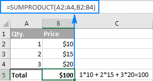
Here is what's going on under the hood in terms of math:
- The formula takes the 1st number in the 1st array and multiplies it by the 1st number in the 2nd array, then takes the 2nd number in the 1st array and multiplies it by the 2nd number in the 2nd array, and so on.
- When all of the array elements are multiplied, the formula adds up the products and returns the sum.
In other words, our SUMPRODUCT formula performs the following mathematical operations:
=A2*B2 + A3*B3 + A4*B4
Just think how much time it could save you if your table contained not 3 rows of data, but 3 hundred or 3 thousand rows!
Tip. If you want to only multiply the numbers in each row without adding up the products, then use one of the formulas to multiply columns in Excel.
How to use SUMPRODUCT in Excel - formula examples
Multiplying two or more ranges together and then summing the products is the simplest and most obvious usage of SUBTOTAL in Excel, though not by far the only one. The real beauty of the Excel SUMPRODUCT function is that it can do far more than its stated purpose. Further on in this tutorial, you will find a handful of formulas that demonstrate more advanced and exciting uses, so please keep reading.
SUMPRODUCT with multiple criteria
Usually in Microsoft Excel, there is more than one way to accomplish the same task. But when it comes to comparing two or more arrays, especially with multiple criteria, SUMPRODUCT is the most effective, if not the only, solution. Well, either SUMPRODUCT or array formula.
Assuming you have a list of items in column A, planned sale figures in column B, and actual sales in column C. Your goal is to find out how many items have made less sales than planned. For this, use one of the following variations of the SUMPRODUCT formula:
=SUMPRODUCT(--(C2:C10<B2:B10))
or
=SUMPRODUCT((C2:C10<B2:B10)*1)
Where C2:C10 are real sales and B2:B10 are planned sales.
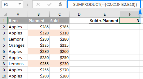
But what if you had more than one condition? Let's say, you want to count how many times Apples performed worse than planned. The solution is to add one more criterion to the SUMPRODUCT formula:
=SUMPRODUCT(--(C2:C10<B2:B10), --(A2:A10="apples"))
Or, you can use the following syntax:
=SUMPRODUCT((C2:C10<B2:B10)*(A2:A10="apples"))
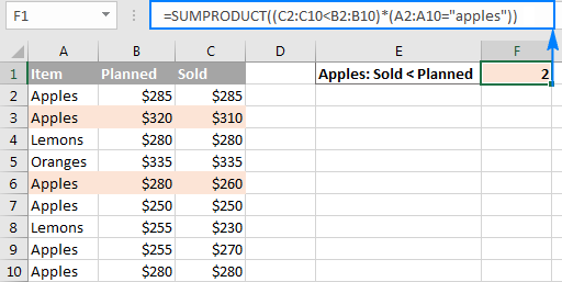
And now, let's take a minute and understand what the above formulas are actually doing. I believe it is a worthy time investment because many other SUMPRODUCT formulas work with the same logic.
How SUMPRODUCT formula with one condition works
For starters, let's break down a simpler formula that compares numbers in 2 columns row-by-row, and tells us how many times column C is less than column B:
=SUMPRODUCT(--(C2:C10<B2:B10))
If you select the portion (C2:C10<B2:B10) in the formula bar, and press F9 to view the underlying values, you will see the following array:
![]()
What we have here is an array of Boolean values TRUE and FALSE, where TRUE means the specified condition is met (i.e. a value in column C is less than a value in column B in the same row), and FALSE signifies the condition is not met.
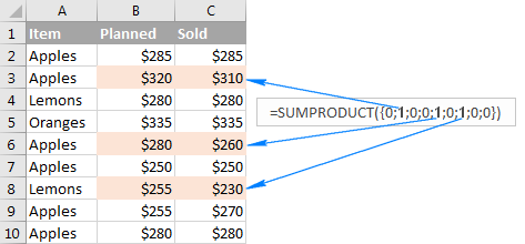
The double negative (--), which is technically called the double unary operator, coerces TRUE and FALSE into ones and zeros: {0;1;0;0;1;0;1;0;0}.
Another way to convert the logical values into the numeric values is multiple the array by 1:
=SUMPRODUCT((C2:C10<B2:B10)*1)
Either way, since there is just one array in the SUMPRODUCT formula, it simply adds up 1's in the resulting array and we get the desired count. Easy, isn't it?
How SUMPRODUCT formula with multiple conditions works
When an Excel SUMPRODUCT formula contains two or more arrays, it multiplies the elements of all the arrays, and then adds up the results.
As you may remember, we used the following formulas to find out how many times the number of real sales (column C) was less than planned sales (column B) for Apples (column A):
=SUMPRODUCT(--(C2:C10<B2:B10), --(A2:A10="apples"))
or
=SUMPRODUCT((C2:C10<B2:B10)*(A2:A10="apples"))
The only tech difference between the formulas is the method of coercing TRUE and FALSE into 1 and 0 - by using the double unary or multiplication operation. As the result, we get two arrays of ones and zeros:
![]()
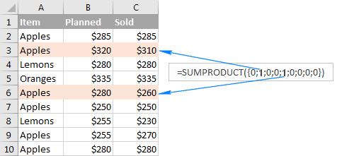
The multiplication operation performed by SUMPRODUCT joins them into a single array. And since multiplying by zero always gives zero, 1 appears only when both conditions are met, and consequently only those rows are counted:
Conditionally count / sum / average cells with multiple criteria
In Excel 2003 and older versions that did not have the so-called IFs functions, one of the most common uses of the SUMPRODUCT function was to conditionally sum or count cells with multiple criteria. Beginning with Excel 2007, Microsoft introduced a series of functions specially designed for such tasks - SUMIFS, COUNTIFS and AVERAGEIFS.
But even in the modern versions of Excel, a SUMPRODUCT formula could be a worthy alternative, for example, to conditionally sum and count cells with the OR logic. Below you will find a few formula examples that demonstrate this ability in action.
1. SUMPRODUCT formula with AND logic
Supposing you have the following dataset, where column A lists the regions, column B - items and column C - sales figures:
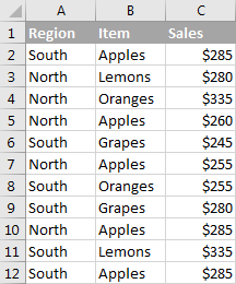
What you want is get the count, sum and average of Apples sales for the North region.
In Excel 2007 and higher, the task can be easily accomplished by using a SUMIFS, COUNTIFS and AVERAGEIFS formula. If you are not looking for easy ways, or if you are still using Excel 2003 or older, you can get the desired result with SUMPRODUCT.
- To count Apples sales for North:
=SUMPRODUCT(--(A2:A12="north"), --(B2:B12="apples"))or
=SUMPRODUCT((A2:A12="north")*(B2:B12="apples")) - To sum Apples sales for North:
=SUMPRODUCT(--(A2:A12="north"), --(B2:B12="apples"), C2:C12)or
=SUMPRODUCT((A2:A12="north")*(B2:B12="apples")*C2:C12) - To average Apples sales for North:To calculate the average, we simply divide Sum by Count like this:
=SUMPRODUCT(--(A2:A12="north"), --(B2:B12="apples"), C2:C12) / SUMPRODUCT( --(A2:A12="north"), --(B2:B12="apples"))
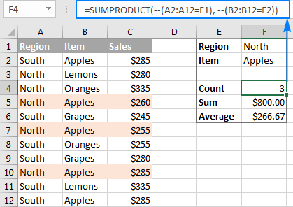
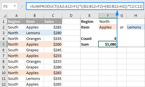
To add more flexibility to your SUMPRODUCT formulas, you can specify the desired Region and Item in separate cells, and then reference those cells in your formula like shown in the screenshot below:
How SUMPRODUCT formula for conditional sum works
From the previous example, you already know how the Excel SUMPRODUCT formula counts cells with multiple conditions. If you understand that, it will be very easy for you to comprehend the sum logic.
Let me remind you that we used the following formula to sum Apples sales in the North region:
=SUMPRODUCT(--(A2:A12="north"), --(B2:B12="apples"), C2:C12)
An intermediate result of the above formula are the following 3 arrays:
![]()
- In the 1st array, 1 stands for North, and 0 for any other region.
- In the 2nd array, 1 stands for Apples, and 0 for any other item.
- The 3rd array contains the sales numbers exactly as they appear in cells C2:C12.
Remembering that multiplying by 0 always gives zero, and multiplying by 1 gives the same number, we get the final array consisting of the sales numbers and zeros - a sales number appears only if the first two arrays have 1 in the same position, i.e. both of the specified conditions are met; zero otherwise:

Adding up the numbers in the above array delivers the desired result - the total of the Apples sales in the North region.
Example 2. SUMPRODUCT formula with OR logic
To conditionally sum or count cells with the OR logic, use the plus symbol (+) in between the arrays.
In Excel SUMPRODUCT formulas, as well as in array formulas, the plus symbol acts like the OR operator that instructs Excel to return TRUE if ANY of the conditions in a given expression evaluates to TRUE.
For example, to get the count of all Apples and Lemons sales regardless of the region, use this formula:
=SUMPRODUCT((B2:B12="apples")+(B2:B12="lemons"))
Translated into plain English, the formula reads as follows: Count cells if B2:B12="apples" OR B2:B12="lemons".
To sum Apples and Lemons sales, add one more argument containing the Sales range:
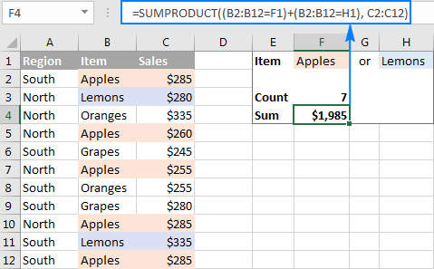
=SUMPRODUCT((B2:B12="apples")+(B2:B12="lemons"), C2:C12)
The following screenshot shows a similar formula in action:
Example 3. SUMPRODUCT formula with AND as well as OR logic
In many situations, you might need to conditionally count or sum cells with AND logic and OR logic at a time. Even in the latest versions of Excel, the IFs series of functions is not capable of that.
One of the possible solutions is combining two or more functions SUMIFS + SUMIFS or COUNTIFS + COUNTIFS.
Another way is using the Excel SUMPRODUCT function where:
- Asterisk (*) is used as the AND operator.
- Plus symbol (+) is used as the OR operator.
To make things easier to understand, consider the following examples.
To count how many times Apples and Lemons were sold in the North region, make a formula with the following logic:
=Count If ((Region="north") AND ((Item="Apples") OR (Item="Lemons")))
Upon applying the appropriate SUMPRODUCT syntax, the formula takes the following shape:
=SUMPRODUCT((A2:A12="north")*((B2:B12="apples")+(B2:B12="lemons")))
To sum Apples and Lemons sales in the North region, take the above formula and add the Sales array with the AND logic:
=SUMPRODUCT((A2:A12="north")*((B2:B12="apples")+(B2:B12="lemons"))*C2:C12)
To make the formulas a bit more compact, you can type the variables in separate cells - Region in F1 and Items in F2 and H2 - and refer to those cells in your formula:
SUMPRODUCT formula for weighted average
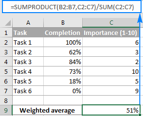
In one of the previous examples, we discussed a SUMPRODUCT formula for conditional average. Another common usage of SUMPRODUCT in Excel is calculating a weighted average where each value is assigned a certain weight.
The generic SUMPRODUCT weighted average formula is as follows:
Assuming that values are in cells B2:B7 and weights are in cell C2:C7, the weighted average SUMPRODUCT formula will look like this:
=SUMPRODUCT(B2:B7,C2:C7)/SUM(C2:C7)
I believe at this point you won't have any difficulties with understanding the formula logic. If someone needs a detailed explanation, please check out the following tutorial: Calculating weighted average in Excel.
SUMPRODUCT as alternative to array formulas
Even if you are reading this article for informational purposes and the details are likely to fade away in your memory, remember just one key point - the Excel SUMPRODUCT function deals with arrays. And because SUMPRODUCT offers much of the power of array formulas, it can become an easy-to-use replacement for them.
What advantages does this gives to you? Basically, you will be able to manage your formulas an easy way without having to press Ctrl + Shift + Enter every time you are entering a new or editing an existing array formula.
As an example, we can take a simple array formula that counts all characters in a given range:
and turn it into a regular formula:
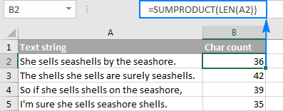
For practice, you can take these Excel array formulas and try to re-write then using the SUMPRODUCT function.
Excel SUMPRODUCT - advanced formula examples
Now that you know the syntax and logic of the SUMPRODUCT function in Excel, you may want to learn more sophisticated and more powerful formulas where SUMPRODUCT is used in liaison with other Excel functions.
Practice workbook for download
Excel SUMPRODUCT examples (.xlsx file)
 by
by
234 comments
could you pls solve me this , this is data sourse
Red Light Green Light Yellow Light Month
01/01/2024 4 5 7 Jan
05/01/2024 6 9 4 Jan
01/03/2024 7 3 4 Mar
this just a sample of a big data, the result should be:
Red Light Green Light Yellow Light Light
Jan (sum of red light for Jan) (sum of Green light for Jan) (sum of Yellow light for Jan) (sum of light for Jan based on partial text)
Mar
How to solve this pls
Hi! To find the sum of the values in a column by condition for a month, you can use SUMIF or SUMIFS formula. You can find the examples and detailed instructions here: How to use SUMIF function in Excel and Excel SUMIFS and SUMIF with multiple criteria. For example:
=SUMIF(E2:E100,"Jan",B2:B100)
or
=SUMIFS(B2:B100,A2:A100,">=01/01/2024",A2:A100,"<=31/01/2024")
Or you can use SUMPRODUCT formula as described in the article above. For example:
=SUMPRODUCT(B2:B100*(E2:E100="Jan"))
I am looking to sum the values in a cell column 'AN' based on the conditions in my original formula below.
my current formula is ;
=COUNTIFS(Report!$I$6:$I$1176,'Data validation'!$D$7,Report!$H$6:$H$1176,">"&TODAY()-31,Report!$AL$6:$AL$1176,"*US*")
i would like to extend this from a countifs to a Sum of the values in column AN for the conditions above.
many thanks
Hi! Use the SUMIFS function with the same conditions you applied in your formula. You can find the examples and detailed instructions here: Excel SUMIFS and SUMIF with multiple criteria – formula examples. The formula might look as follows:
=SUMIFS(AN6:AN1176,Report!$I$6:$I$1176,'Data validation'!$D$7,Report!$H$6:$H$1176,">"&TODAY()-31,Report!$AL$6:$AL$1176,"*US*")
fantastic, really appreciate your advice and website content. thank you
I am trying to use SUMIFS with two criteria from two sheets. One is MMM-YY and second is "Direct" or "Indirect" and it does not return the correct sum.
Hi! I don't know what formula you are using. I don't have an example of your data. Unfortunately, this information is not enough to give you any advice. I recommend reading and studying these instructions carefully: Excel SUMIFS and SUMIF with multiple criteria – formula examples. Or describe the problem in more detail.
Hi Alexander, Im hoping you can help.
I am thinking I will need to use SUMPRODUCT Formula however, please tell me if I'm wrong.
I have C5 (value) D5 (Month) E5 (markup percent)
I then have F3 (January) G3 (February) H3 (March) etc.
I need F5 to pickup D5 and work out the C5 x E5 /100
F5 being specific to F3 'January' so needing to match that.
Hi! I’m not sure I got you right since the description you provided is not entirely clear. I don't know what is written in F5. To calculate the amounts for January, you can try this formula:
=SUMPRODUCT((C5:C10)*(D5:D10=1)*E5:E10/100)
If this does not help, explain the problem in detail.
Hello Alexander, I am attempting to find the average age of my clients, weighted by revenue they produce. I have attempted to use SUMPRODUCT with and IF, AND qualifier, to select for just those clients on a certain code (denoted in cell B14) and by a second qualifier that is in cell b11. Here is what I have:
SUMPRODUCT(IF(AND('Client List'!$D$2:$D$1000='7TEC'!$B$14)('Client List'!L2:L1000='7TEC'!B11),(('Client List'!$K$2:$K$1000*'Client List'!$G$2:$G$1000)/'7TEC'!F$26)))
When I calculate, I keep getting zero. Any help you might provide in sumproduct calculations with two qualifying conditions would be greatly, greatly appreciated.
Hi! I can't check a formula that contains unique references to your data, which I don't have. Note that there is no comma between AND conditions in the formula.
I am currently using =SUMPRODUCT(($F$3:$F$8="A")*($E$3:$E$8="22/02/24)*$G$3:$G$8) for daily Total. But I'm looking to create another not monthly, Meanting I need to change the single date to a date range, for example >01/02/24 <29/02/22.
Would you be able to assist?
Hi! Add another condition as described in the article above. The date can be set using the DATE function.
=SUMPRODUCT(($F$3:$F$8="A")*($E$3:$E$8>=DATE(2024,2,1))*($E$3:$E$8<=DATE(2024,2,29))*$G$3:$G$8)
To find the sum by condition, you can also use the COUNTIFS function. You can find the examples and detailed instructions here: How to use SUMIFS in Excel - formula examples.
=SUMIFS($G$3:$G$8,$F$3:$F$8,"A",$E$3:$E$8,">="&DATE(2024,2,1),$E$3:$E$8,"<="&DATE(2024,2,29))
Hello,
I am searching for a suitable formula to split out headcount between different shows in our organization. I feel like sumproduct or a version of it would be what I need but I cant figure it out.
Normally I would use countifs to obtain headcount information for a specific week to show HC under specific show/department. But it only works if I have employee scheduled under one show.
Is there any version of sumproduct that would recognize how many "*/*" there is in a schedule and say if someone is scheduled under show1/show5/show8, then formula assigned 0.33 for every of the shows within that week. And if there was no / i nthe text, it would be 1 as a headcount.
Thanks,
Mi.
Hi! You can count the number of "/" characters in a text string using the formula below. Consecutively extract each character from the text using the MID function and compare it with the "/". Use the SUM function to count the matches.
=SUM(--(MID(A1,ROW(A1:A100),1)="/"))
Thank you Alexander,
I was thinking about it, but how will this count actual shows? Because the % depends on how many shows someone is scheduled between. but then the actual show code determines where either full headcount or partial goes to.
Example:
Column_1 | Column_2 | Column_3 | Column_4
Employee ID | Department | 11.27.2023 | 12.4.2023
123456 | HR | Dev/HR | HR
123455 | IT | Dev/Training | DEV
123466 | DEV | Dev/Training | DEV
123465 | HR | HR/Training | Training
In this case I have 4 employees - thus should have 4 HC each week.
SHOW(TASK)| 11.27 | 12.4
HR | 1 | 1
DEV | 1.5 | 2
Training | 1.5 | 1
But using =SUM(--(MID(A1,ROW(A1:A100),1)="/")) it will only show me 1 and 0 depending on how many "/" there were in a specific week.
Hi! The formula I sent to you was created based on the description you provided in your first request. However, as far as I can see from your second comment, your task is now different from the original one.
Try this formula:
=SUM((ISNUMBER(SEARCH($H$1,C1:C4)))/(ISNUMBER(SEARCH("/",C1:C4))+1))
For more information, please read: How to find substring in Excel
H1 -- "HR"
Thank you for a suggestion. Unfortunately it did not work.. It gives me "Error!
Is there any way I could upload an excel example?
In the "Conditionally count / sum / average cells with multiple criteria" section, what if instead of "apples" you had multiple colors in front of the word "apple" in the same cell; so "Red Apples", "Golden Apples", etc. How could you write the formula to tally any version of the word "apple" that occurs?
In a regular SUMIF you can do this with quote star word star quote, eg. SUMIF($B$2:$B$12,"*Apples*",$C$2:$C$12), however I tried this with SUMPRODUCT and it did not work. Any suggestions?
Hi! If I got you right, the formula below will help you with your task:
=SUMPRODUCT(--ISNUMBER(SEARCH("apple",B2:B12)),C2:C12)
For more information, please read: How to find substring in Excel
That worked! Thank you!
Dear Sir,
Can you help me to fix the sumproduct result to get (i.e.32.49%) mentioned below working.
I have want to get the sumproduct function with following serious
Project Cost (A1); Variation(B1); % of Profit(C1)
50000 3000 25%
80000 8000 37%
Total 130000 11000 32.49% (How to get this result 32.49% in function)
Thanks & Regards,
Sunil Pinto
Hi! I assume you want to get a weighted average value. I couldn't get the result you want, but you can try these formulas yourself: How to calculate weighted average in Excel.
I have a table where several values are generated daily, such as is shown (actual data extends to many more days)
1 A B C D E F G .......
2
3 S M T W T F S ........
4
5 3 4 10 4 8 6 6
6 4 7 4 6 4 5 4
7 5 3 10 5 6 3 7
8 6 5 6 8 5 7 8
I would like to create a formula that can find which day's 4 numbers contains
the smallest (and largest) sum, preferably without using a helper cell to post the sums.
In the example above, cells A5:A8 for Sunday (3 4 5 6 = 18) would be smallest,
cells C5:C8 for Tuesday (10 4 10 6 = 30) would be largest.
I would like to have a running account of smallest and largest that
continually updates itself as each day's 4 numbers are added to the array.
If the smallest could be shown, I can figure out the largest from that.
Any help would be greatly appreciated ! Thanks !
Hello
I am not getting the desired outcome with below mentioned formula;
=SUMPRODUCT(SUMIFS(Raw!K:K,Raw!$D:$D,Summary!$F19,Raw!$C:$C,(Summary!$F$5:$F$13)*($E$5:$E$13=TRUE),Raw!G:G,(Summary!$C$19:$C$64)*(Summary!$E$19:$E$64=TRUE)))
In this, (Summary!$C$19:$C$64) is a Text so the product of this array is giving error, Is there any other way to run this condition.
Hi! It is very difficult to understand a formula that contains unique references to your workbook worksheets. Hence, I cannot check its work. But it is not possible to summarize text values.
Hello Again
Please check, I have made it easier to understand
=SUMPRODUCT(SUMIFS($C$2:$C$16,$A$2:$A$16,($F$2:$F$4)*($G$2:$G$4=TRUE),$B$2:$B$16,($H$2:$H$7)*($I$2:$I$7=TRUE)))
In This ($H$2:$H$7) range contains Text, I have entered this formula in J2 Cell. In column 1 there are headers.
Pls refer below data set I have used as an example.
A B C F G H I
92 SD01 10 91 TRUE SD01 TRUE
93 SD01 8 92 FALSE SD02 TRUE
93 SD03 7 93 FALSE SD03 FALSE
91 SD06 10 SD04 FALSE
92 SD03 7 SD05 TRUE
93 SD02 7 SD06 FALSE
92 SD05 5
93 SD05 9
92 SD02 10
93 SD03 10
91 SD04 5
91 SD03 7
93 SD04 10
91 SD03 5
92 SD01 8
Hi! In the SUMIFS formula, all ranges must be the same size. We have written about this many times in the blog. The SUMIFS function does not work with arrays. Therefore, you cannot use the formula ($F$2:$F$4)*($G$2:$G$4=TRUE), which returns an array. You multiply "SD01" by TRUE. What result do you expect to get?
Got it, Thanks.
It would be great help if you can suggest any other formula to get the result.
I can't guess what you want to do and what result you need to get.
Sumproduct function SUMPRODUCT(MAX((E2:E10=M2)*(F2:F10))) works for maximum value extraction. If you replace MAX by MIN result is zero.
Is there any non array formula to find the minimum. I am not keen on using MIN IF
Hi! The formula below will do the trick for you:
=SUMPRODUCT(MIN(IF((E2:E10=M2)*(F2:F10)>0,(E2:E10=M2)*(F2:F10),"")))
Hi,
I want to nest a ranged LEFT function into a SUMIFS formula, but am getting either a #SPILL and/or #VALUE error, I believe SUMPRODUCT should help but I'm not sure how. Here is my formula:
=SUMIFS(A1:A100,B1:B100,"B",C1:C100,"C",D1:D100,LEFT(D1:D100,1)="D")
To be clear, I want to return a single value that is the sum of all values in the range A1:A100 that meet three criteria, but excel wants to return 100 #VALUE errors spilling down the sheet. Thoughts?
Thank you!
Hi! As I have written many times before, the SUMIFS function cannot use other functions as arguments. Use the SUMPRODUCT function for your task. Try this formula:
=SUMPRODUCT(A1:A100,--(B1:B100="B"),--(C1:C100="C"),--(LEFT(D1:D100,1)="D"))
I want the offset in it. How will this happen?
=SUMPRODUCT(--(C5="Kalim"),H4-G5+F5+E5-D5)+SUMPRODUCT(--(C5="Ali Sir"),H4+G5+F5+E5)
Sorry, it's not quite clear what you are trying to achieve.
Hi Ablebits Team:
I have a "SUMPRODUCT with multiple criteria" challenge in Excel:
I have filter criteria in Columns E and F
And I need to calculate the weighted average of the values in Columns S and U.
All columns have the same number of rows.
I can figure out the formula for one criterion using SUMPRODUCT-IF: =(SUMPRODUCT(IF(E$37:E$250000=11,U$37:U$250000*(S$37:S$250000/S$8))))*1000
But I can't figure out the formula in cases where there are two criteria...
Can you help?
Thanks in advance...
EP
Hi! There is no standard SUMPRODUCT-IF function in Excel. Explain in detail what you want to do. Give an example of the source data and the desired result.
I recommend reading this guide: How to calculate weighted average in Excel.
=SUMPRODUCT(SUMIF(INDIRECT("'"&'1:31'!&"'!C:C"),"A&P CHECK,INDIRECT("'"&'1:31'!&"'!D:D")))
hi, is this formula correct?
I want to sum Column D in sheets 1 to 31 if the column C contains text "A&P CHECK"
Hi!
Unfortunately, your formula will not work.
In the article 3-D reference in Excel: reference the same cell or range in multiple worksheets you can find list of functions supporting 3D references.
Try to use the recommendations described in this article: SUMIF multiple columns with one or several criteria in Excel. I hope it’ll be helpful.
How would you manage the syntax when pulling data from other workbooks with multiple criteria: sumproduct(--(different workbook sheet1 range = A2)*(different workbook sheet2 range=20),(different workbook range to bring in))
Thank you!
Hi!
If I understand the problem correctly, it will be helpful for you to study this manual: Excel reference to another sheet or workbook (external reference).
Have a sheet with 2500 rows and 42 columns. Utilizes Sort & Filter for the header rows (row3). A summary of what review code meaning is the top row/colums for each review code. I would like that count to dynamically change as the filters are changed.
I've tried the functions below but have issues with each.
SUMPRODUCT(COUNTIF(B3:B7,"*04a*"))*(SUBTOTAL(3,OFFSET(B4,ROW(B3:B7)-MIN(ROW(B3:B7)),0))) but gives #SPILL errors when used in columns that has data below it.
SUMPRODUCT((B4:B7="04a")*(SUBTOTAL(3,OFFSET(B4,ROW(B4:B7)-MIN(ROW(B4:B7)),0)))) works but only if I give it exact match criteria. Any use of wildcards results in 0 record count being returned. In the sample data provide, row5 and row6 contain 04a so the result should be 2 which matches the Filter selection.
Is there a way to have the header summary dynamically update when the filter is changed. I frequently filter on items that may be embedded with the other review codes so need a contains text solution.
c1 c2 c3 etc..
r1 01a count based on applied filter 04a count based on applied filter 04f count based on applied filter etc…
r2
r3 review code product State
r4 01a Apple FL
r5 04a Orange FL
r6 01a 04a 10a 12a Apple AZ
r7 04f 10a Cherries CA
Hello!
To search for a text string in a cell, instead of (B4:B7="*04a*"), use the expression
ISNUMBER(SEARCH("04a",B4:B7))
SUMPRODUCT((--ISNUMBER(SEARCH("04a",B4:B7))) * (SUBTOTAL(3,OFFSET(B4,ROW(B4:B7)-MIN(ROW(B4:B7)),0))))
This should solve your task.
Works like a champ!
Looks so simple now that I see the solution
Thank you again
Hello to all
I am trying to return the sum of the value from a specific column based on multiple criteria in a row and/ or column.
As an ex-example:
Database
Column A Column B Column C Column D
Row month date Type Project name Sales
Row 1 01/31/2022 Revenue1 Kansas 100
Row 2 03/22/2023 Revenue2 Texas 26
Row 3 01/23/2023 Revenue1 Kansas 150
Row 4 01/31/2023 Revenue1 Kansas 10
I need to create the sumproduct condition that will return the value 260, which is the sum Row 1, Row 3, and Row 4 based on the below criteria:
Q1-2023 (which will collect 01/23/2023 and 01/31/2023), Revenue1, Kansas as the project name.
I tried with the SUMIFS but the formula is static through a specific column.
Thank you in advance for your help.
Hello!
Please read the above article carefully. To calculate the sum by conditions, you can find useful information in this article - Excel SUMIFS and SUMIF with multiple criteria.
=SUMPRODUCT(--(A1:A4>=DATE(2023,1,1)),--(A1:A4<=DATE(2023,3,31)),--(B1:B4="Revenue1"),--(C1:C4="Kansas"),D1:D4)
=SUMIFS(D1:D4,A1:A4,">="&DATE(2023,1,1),A1:A4,"<="&DATE(2023,3,31),B1:B4,"Revenue1",C1:C4,"Kansas")
Thank you, Alexander,
Thank you for the recommendation and guidance; however, how can I get the formula to search first a specific title of a column and then have the research done?
As an example, the column "type" in the current formula is selected as an array (B1:B4="Revenue1) . Can it be possible to have a condition that search first a specific labeled column (in this case, "type" and then at this time indirectly take a chosen additional criteria in this now found column ("Revenue1") and continue the formula as you explained (-(C1:C4="Kansas"),D1:D4))
Thank you again for all your help.
JP
Muchas gracias, me fue de mucha utilidad
Hi, this formula:
=SUMPRODUCT(--ISNUMBER(SEARCH(B3&" for ",Description)))*Cost
is returning required value. I want to add a second criteria to return value based on date range. So I changed formula to:
=SUMPRODUCT(--(ISNUMBER(SEARCH(B3&" for ",Description))),--(Date,">="&$D$1,Date,"<="&EOMONTH($D$1,0))*Cost)
Unfortunately, formula is returning #VALUE. It looks like the date part of formula is generating the #VALUE error. Could you take a look please?
Your help is greatly appreciated.
Hello!
Use this example to add a date range to the SUMPRODUCT function
=SUMPRODUCT(--(A1:A10>=$D$1),--(A1:A10<=EOMONTH($D$1,0)))
I hope it’ll be helpful.
Thanks for help.
Hello, I am interested in adding a formula to my excel to reflect if this cells has a specific month or date range, to sum this column.
ex:
A B C D E
CC-234-10-31-2022 VIROLOGY 101001 VIROLO 10/31/2022 235.17
CC-234-10-12-0222 PARASITOLOGY 101001 PARAST 10/12/2022 324.00
CC-234-10-11-0222 PARASITOLOGY 101001 PARAST 10/11/2022 324.00
CC-234-10-10-0222 PARASITOLOGY 101001 PARAST 10/10/2022 324.00
CC-234-10-09-0222 PARASITOLOGY 101001 PARAST 10/9/2022 324.00
CC-234-10-03-0222 PARASITOLOGY 101001 PARAST 10/3/2022 324.00
if column D has a date between 10/1/2022 and 10/31/2022 (or just the month 10; whichever is easier), sum up column E.
Hello!
To calculate the sum of values in a date range, use this tutorial: SUMIF with dates.
This should solve your task.
Is it possible to use the filter feature to replace the condition cells, eg instead of getting the condition from E1:H5 above, replace with filter result from A1:C1
Meaning I would like to have sumproduct but my conditions are very dynamic
Hi!
The information you provided is not enough to understand your case and give you any advice, sorry.
Manager Name : Daily Attendance'!$F$4:$F$154
Dates: Daily Attendance'!$G$4:$AK$4
B3=Manager Name, B5= date
Daily attendance of the resources marked as (Present(P), Absent(A), Approved Leave(AL), Unplanned Leave(UL) etc..) in Daily Attendance'!$g$5:$AK$154 range
=SUMPRODUCT(('Daily Attendance'!$F$4:$F$154=B5)*('Daily Attendance'!$G$4:$AK$4=$B$3),(COUNTIFS(G$4:G$154,"P")+COUNTIFS(G$4:G$154,"PNS")))
Here, (COUNTIFS(G$4:G$154,"P")+COUNTIFS(G$4:G$154,"PNS"))) this is not a number value hence formula isn't working.
Kindly help me to get count of attendance marked from Daily Attendance'!$g$5:$AK$154 range for a particular manager for a specific date
Hi!
It is very difficult to understand a formula that contains unique references to your workbook worksheets. If you have a specific question about the operation of a function or formula, I will try to answer it.
Sorry, below is the range from which I am trying to get the count of Present (P) + PNS
(COUNTIFS('Daily Attendance'!$G$4:$AK$154,"P")+COUNTIFS('Daily Attendance'!$G$4:$AK$154,"PNS")))
Thank you for your quick response Alexander !
Hello. I want to use sumproduct with multiple criteria but the value of one criterion might be located in multiple rows. Ideally I would like to use something such as :
=SUMPRODUCT(($C$50:$DQ$50="Theoretical")*($C$11:$DQ$122=$H8)*($H$11:$H$122=Summary!D$6),'Sheet1 (62)'!$C$11:$DQ$122)
but the ($C$11:$DQ$122=$H8) makes the formula to give 0. Is there any other way of searching that H8 value in multiple rows and columns?
Hello!
All ranges in the SUMPRODUCT formula must be the same size. You cannot multiply matrices with different numbers of rows or columns.
Hello again. They have the same range. The table is from C11 till DQ122. My question is if it is possible to apply criteria within many columns AND rows instead for either rows or columns
Hi!
Are $C$50:$DQ$50 and $C$11:$DQ$122 and $H$11:$H$122 have the same range?
But when I put the formula below it is not giving an error:
=SUMPRODUCT(($C$50:$DQ$50="Theoretical")*($C$11:$DQ$11=$H7)*($H$11:$H$122=D$2),$C$11:$DQ$122) while the H$11:H$122 is not the same as C$50:DQ$50. But they refer to only one column or only one row
Hi!
I am not sure I fully understand what you mean. Please clarify your issue or provide additional information to understand what you need.
Hi again,
Thanks for your help. I found another way of dealing with that issue. Basically, I have some sheets with tables similar to the table below. I was setting a formula such as =SUMPRODUCT(($A$1:$F$8)*($A$1:$A$8=$A2)*($A$1:$F$8=B1)) in order to find the 1a,2a,3a etc values. The issue is that the rows with the header "6,7,8" are not at the same row always. Therefore, I cannot set the row 5 as the range for my criterion. The criterion ($A$1:$F$8=B1) is giving an error as it needs to be only 1 row instead of a range of rows. I still don't know though if something like that is possible but I hope my problem is more clear now.
1 2 3 4 5
a 1a 2a 3a 4a 5a
b 1b 2b 3b 4b 5b
c 1c 2c 3c 4c 5c
6 7 8
a 6a 7a 8a
b 6b 7b 8b
c 6c 7c 8c
Hello!
I'm not sure I fully understand your issue. Maybe this article will be helpful: INDEX MATCH MATCH in Excel for two-dimensional lookup.
Hello!
I need some help also :)
I have a huge table with:
Columns:
- two columns with parameters: ColSupplier = supplier, ColProject = Project
- many columns with weekly production outputs (1 column / week) - so I have 3 lines of parameters to define one column: year (LinYear) + quarter (LinQtr) + week number
I need to sum up per supplier and per project the production output by quarter or by year.
I have managed to reach out to the right "first cell" cells with "INDEX/MATCH function":
=INDEX(DataTable,MATCH(1,(ColSupplier="Supplier 1"*(ColProj="Project A"),0), MATCH(1,(LinYear="2023")*(LinQtr="Q2"),0)))
But I need to sum up all production outputs over the full quarter (up to 13 weeks = 13 columns), and not only revert the first weekly output Excel is finding. I try adding SUM in front of INDEX but it does not work.
Thanks in advance for your support!
Best regards
Serge
Hello!
I hope this example formula will show you the solution using your data. Multiply the conditioned matrix and the data matrix and use the SUM function to calculate the quarterly sum.
=SUM(((A4:A10="Supplier 1")*(B4:B10="Project A")) * ((C2:G2="Q2")*(C1:G1=2023)) * C4:G10)
I hope I answered your question. If something is still unclear, please feel free to ask.
Great, it is working perfectly, thanks a lot!
I have hundreds of rows of data on a worksheet. I can use filters to glean the counts of items, but I have used sumproduct to do this in the past. Unfortunately, I lost the complex formula string when I changed computers. I am attempting to get a count of items that match multiple criteria in the columns. For example, see below, I am attempting to gather a count of items using the Name, Class, Location, and Style. I recall using "--" between the SUMPRODUCT functions to narrow down the retrieved data and displayed it as the output. For example, using SUMPRODUCT I would like to get the count of Names that are a specific Location that have a specific Size. Thank you ...
Name | Class | Location | Size
Joe | Third | AZ | Large
Bill | First | NJ | Med
Francis | Third | AZ | X-Large
Harry | First | NV | Med
Hello!
If I understand your task correctly, the following tutorial should help: Conditionally count / sum / average cells with multiple criteria.
I hope it’ll be helpful. If something is still unclear, please feel free to ask.
Hello Alexander!
Thank you! The tutorial provided the information required to complete the task in Excel.
Hello!
I have multiple columns and rows that I need a count for. Going by the above example, I was looking for a formula / method that counts the below
1. ALL regions (North + South) and ONLY Lemons
2. ONLY North region and ALL items (Apples + Lemons + Oranges)
3. ALL regions and ALL items
The input requirement of region and fruit specification (whether region is All, North, or South; whether item is All, Apples, Lemons, Oranges) can be flexible using a filter.
Thanks for your help!
Hello Alexander,
I need help please.
I have 3 columns (A-B-C):
A has 12 records both text and numerical;
B has 10,000 records TEXT format;
C has 10,000 records TEXT and NUMERIC format;
I need to COUNT records in the column "B", IF column "C" MATCH column "A". As you can see, both Column "B" and "C" have a direct correlation (in other words it is one table).
Please note, the COUNT formula cannot be referenced each individual "CELL" 12 times from the column "A". I will need to copy the formula to other files, and sometimes there will be 5 records in column "A", sometimes 15, or even 25. The idea for this formula is to change the "RANGE" only, based on column "A" records from one file to another.
Any help is greatly appreciated.
Hello!
To count the number of records by multiple criteria, use the SUMPRODUCT function:
=SUMPRODUCT(--ISNUMBER(MATCH($C$1:$C$100,$A$1:$A$30,0)), --($B$1:$B$100<>""))
Hope this is what you need.
Unfortunately, I could not find any simple examples using MATCH with SUMPRODUCT.
Thank you Alexander, your formula worked.
Hello all,
I'm trying to do a stack ranking based on performance that are weighted differently. I have 9 measurements that fall into three groupings, Management, Wallet share, and quality. Should I sum the stack ranking of each grouping to get the weighted score and then use the sumproduct formula so that I can get a total stack ranking?
The weighting is 30% Management, 30% wallet, and 40% for quality.
Hello!
Try to use the recommendations described in this article: How to calculate weighted average in Excel. I hope I answered your question. If something is still unclear, please feel free to ask.
Thank You very much.
Hello - I am trying to calculate the 75th percentile of a weighted average. When I combine the percentile and sumproduct, it seems to only return the sumproduct. The values I am using are 1) column with number of incumbents; and 2) the salary for each. In the example below, I believe the answer should be $118,206, but sumproduct keeps returning the answer of $123,278 - this is the weighted average, but I need the 75th percentile of the weighted average. Thanks.
Inc Salaries
17 111,043
1 111,298
1 118,206
1 135,200
1 151,388
1 162,136
1 163,865
1 166,462
1 185,661
Hello!
You can only calculate the percentile from one column of values. Use PERCENTILE function.
You can also use this formula.
=RANK.EQ(B1,$B$1:$B$9,1)/COUNT($B$1:$B$9)
Write it in C1 and copy it down the column to calculate all rank percentiles.
I am trying to figure out how to use the SUMPRODUCT formula to count the number of times an event happens within each month (JAN-DEC). If the value from another sheet cites FRONT (Front door), it will add it as part of a total within that month
=SUMPRODUCT((Data!C662:C2002="FRONT"))
OR
=SUMPRODUCT((MONTH(Data!A662:A2002)=1)*(YEAR(Data!A662:A2002)=2022)*(Data!E662:E2002="FRONT"))
Hello!
You are making mistakes in the syntax of the SUMPRODUCT function. Read carefully the first paragraph of this article. Also convert logical expressions to numbers. This is also described above.
=SUMPRODUCT(--(MONTH(Data!A662:A2002)=1),--(YEAR(Data!A662:A2002)=2022),--(Data!E662:E2002=”FRONT”))
Do you have dates and text in the same column?
Hi sir,
I'm trying to use sumproduct formula as vba code putting values in place of cell reference, but it's not working.
Can you tell me best way using values
18 37 422.73
1 2 1006.08
2 1 811.62
3 2 1352.71
Hi - I am trying to do a sumproduct of A and C plus a sumproduct of 50% of the values in B and C, but I do not want to create a new column showing the 50%. The answer with the numbers above would be 24,881.695. I really hope this is possible!! THANK YOU!
I'm so sorry - I read this and it confused me. Trying again! :)
18 37 422.73
1 2 1006.08
2 1 811.62
3 2 1352.71
I want to do
sumproduct($A$1:$A$4,$C$1:$C$4)+sumproduct($C$1:$C$4,((0.5*$B$1:$B$4))
but this gives an answer I do not expect (21,444.89) instead of 24,881.695.
Hi!
Please try the following formula:
=SUMPRODUCT(A1:A4,C1:C4) + 0.5*SUMPRODUCT(B1:B4,C1:C4)
I hope it’ll be helpful.
THANK YOU!!
how come ther is no goto command in spreadsheets for exaple
cell a1 input a1
cell a2 if a1 = "home" the goto d1
cell c1 'go
cell c1 c2 = a1
answer
go home
how come we do not have that formulas in spreadshet
Hi!
For conditional calculations, you can use the IF function.
Or use VBA language.
Hello,
Type Sub Code Amount Product
Cost 100 20 A
Sale 100 30 A
Cost 200 40 A
Sale 200 50 A
Sale 300 60 B
I am trying to divide Cost/Sale to find the Percentage for a product group but by each sub code. For example Product A, Sub Code 100: 20/30 + Product A, Sub Code 200: 40/50 and then get the total percentage. I am able to do the divide for the total amount by Product, but I want the divide function to run for each sub code separately and then add it to get to the total Percentage
Hello!
The location of your data makes it very difficult to do the calculations you need.
You can get the corresponding Sale values in column E using the INDEX+MATCH formula:
=INDEX($C$2:$C$6,MATCH(D2&B2&"Sale",$D$2:$D$6&$B$2:$B$6&$A$2:$A$6,0))
After that, you can divide the desired values from column C by column E, and also calculate percentages.
Hi, I think this one might be easy for you, on my side I have been trying for some times now. I would like to create a SUM formula that I can drag down over hundreds of rows that could SUM some figures from the same column depending of the title of this collumn and what is written in the rows. I am not so sure if sumproduct if the best, I would like not to use Sumifs as it would be unreadable and multiple lines of formulas.
Let's imagine;
Collumn A : Shop 1, Shop 2, Shop 3
Collumn B : pear, apple, cherry, apple, cherry, orange, pear
Column C : small, medium, big, small, medium, big, huge.
collumn D : 1st year
Collumn E : 2nd year
Collumn F : 3rd year
collumn G : 4th year
For the rows Collumn A to C, it would be as described: shop, product, size (over 1xxx rows)
and Collumn D to G we will have the quantities sold. (historical TAB that can't be upgraded easily...)
Then, what I would like is in another TAB and in 1formula, to sum the figures depending of the year the product, the size and the shop.
Again, I know I could use sumifs (I think ><), but I would like to avoid that. maybe sumproduct is not the best, wish you could help me on this one.
Thank you very very much for your help and time.
Remy
Hello!
If you want to sum values based on a column heading, then I recommend using a pivot table. There, on a separate sheet, you can choose which column you want to summarize and by what criteria.
Hi,
Thank you for your answer, I will try that.
Hello,
I am using the following formula =SUMPRODUCT(--ISNUMBER(SEARCH(Sheet2!$D$82:$D$5523,C3)))>0
I have column C in which I have one or more email addresses delimited with ";". With my formula I am able to check if one of these emails in each cell is used in another Sheet2!$D$82:$D$5523. This seems working well, I am getting true if email exists.
Now I am blocked, I would like to get the value of another column in Sheet2 that matches my search.
Any Idea?
Thank you,
Hello!
Sorry, it's not quite clear what you are trying to achieve. Give an example of the source data and the expected result.
It’ll help me understand it better and find a solution for you.
I want to count number employee who are at 25th,50th,75th percentile of a salary range which i have bifurcated Role wise and experience band wise. Below is the formula which is returning zero as answer kindly help.
1)G:G is Deaprtment Code
2)K:K is Experience Band Code
3) M:M is Designation Code
4) AN:AN is Salary
=SUMPRODUCT(('Active Internal Salary'!$G$2:$G$2192="SOM")--('Active Internal Salary'!$K$2:$K$2192=$B15)--('Active Internal Salary'!$M$2:$M$2192=$B$1),'Active Internal Salary'!$AN$2:$AN$2192<PERCENTILE('Active Internal Salary'!$AN$2:$AN$2192,0.25))
Hiya
I am trying to work with three separate columns of data, ie.
A B C
Red 31 5
Blue 29 10
Yellow 50 20
Green 29 15
Red 31 50
What I am trying to accomplish is I want to be able to work out for each variable in Column A whether it is equal to 31 in column B and if it is then count those in column C on the same row but exclude everything else?
So as above Red = 55, Blue = 0, Yellow = 0, Green = 0.
I have approximately 60000 lines of data.
Your help is very much appreciated!
Hello!
To find the sum of values across multiple criteria, use the SUMIFS function as described in this tutorial.
This should solve your task.
Great explanation.
I have a tough one for you. I manage our sports team and create teams by handicap.
My table consists of 'team number', 'date', Lname, wins, 'total games' and 'team number'. The table rows are added by date at the end of the table, IE latest date is last.
First: I want the handicaps (Wins/Total Games) for the most current (variable=10) rows by Last Name.
Second: Teams, with Last name, sorted the highest team haandicap.
Working on the first formula is have:
=SUMPRODUCT(--(tblHistory[Total Wins]>0),--(tblHistory[Lname]="lane"),tblHistory[Total Wins]) / (SUMPRODUCT(--(tblHistory[Total Games]>0),--(tblHistory[Lname]="lane"),tblHistory[Total Games]))
Which gives me the total for the table...I only want the last X games of handicap.
Can you help?
Hello!
It is very difficult to understand a formula that contains unique references to your workbook worksheets. Please have a look at this article — Excel LARGE function to get N-th highest value.
Sorry for not being explicit enough.
Here is a pic of what my table look like:
Table headers are:
First Name(fname), Last Name(Lname, Team number (1-6), play date, wins, total games.
I would like to get the last 10 play dates of LName both wins and total games.
No everyone plays so the last play date is mostly different.
The goal is to find the last 10 games played and determine their handicap by summing wins divided by summing total-games.
As from above I can get total-total of played and games for a player buy the range is too large.
Last 10 days will provide a good average.
Hello!
With the FILTER function, you can select rows with the 10 last play dates. Then, with this data, you can do the calculations you want.
You can find the examples and instructions here: How to limit the number of rows returned by FILTER function.
This should solve your task.
Hello,
I appreciate the help to use SUMPRODUCT() to calculate the weighted average (Weight & Cost) but only if the value (Center) is found within a designated range of cells.
In the example below, I would like to obtain the WAvg for Set 1 and Set 2. The actual data set is thousand of entries and hundreds of centers, resulting in numerous Sets. Single entry such as if ="apple" OR "lemon" as shown in the lesson will not be feasible to process the large volume. Is it possible for the conditional statement to be a cell range instead of individual values?
Thank you for the help!
Set 1: Centers 949 and 1200
Set 2: Centers 5300 and 3687
Weight Cost Center
5 12380 949
2 90375 1200
3 38306 1200
4 49073 949
5 41498 5300
6 35196 3687
6 28948 949
5 83636 5300
1 21753 5300
1 53236 1200
Hello!
Add conditions to the SUMPRODUCT formula:
=SUMPRODUCT(A2:A11,B2:B11,--(C2:C11>=949),--(C2:C11<=1200))/SUMPRODUCT(A2:A11,--(C2:C11>=949),--(C2:C11<=1200))
I hope my advice will help you solve your task.