The tutorial explains the essence of Excel logical functions AND, OR, XOR and NOT and provides formula examples that demonstrate their common and inventive uses.
Last week we tapped into the insight of Excel logical operators that are used to compare data in different cells. Today, you will see how to extend the use of logical operators and construct more elaborate tests to perform more complex calculations. Excel logical functions such as AND, OR, XOR and NOT will help you in doing this.
Excel logical functions - overview
Microsoft Excel provides 4 logical functions to work with the logical values. The functions are AND, OR, XOR and NOT. You use these functions when you want to carry out more than one comparison in your formula or test multiple conditions instead of just one. As well as logical operators, Excel logical functions return either TRUE or FALSE when their arguments are evaluated.
The following table provides a short summary of what each logical function does to help you choose the right formula for a specific task.
| Function | Description | Formula Example | Formula Description |
| AND | Returns TRUE if all of the arguments evaluate to TRUE. | =AND(A2>=10, B2<5) |
The formula returns TRUE if a value in cell A2 is greater than or equal to 10, and a value in B2 is less than 5, FALSE otherwise. |
| OR | Returns TRUE if any argument evaluates to TRUE. | =OR(A2>=10, B2<5) |
The formula returns TRUE if A2 is greater than or equal to 10 or B2 is less than 5, or both conditions are met. If neither of the conditions it met, the formula returns FALSE. |
| XOR | Returns a logical Exclusive Or of all arguments. | =XOR(A2>=10, B2<5) |
The formula returns TRUE if either A2 is greater than or equal to 10 or B2 is less than 5. If neither of the conditions is met or both conditions are met, the formula returns FALSE. |
| NOT | Returns the reversed logical value of its argument. I.e. If the argument is FALSE, then TRUE is returned and vice versa. | =NOT(A2>=10) |
The formula returns FALSE if a value in cell A1 is greater than or equal to 10; TRUE otherwise. |
In additions to the four logical functions outlined above, Microsoft Excel provides 3 "conditional" functions - IF, IFERROR and IFNA.
Excel logical functions - facts and figures
- In arguments of the logical functions, you can use cell references, numeric and text values, Boolean values, comparison operators, and other Excel functions. However, all arguments must evaluate to the Boolean values of TRUE or FALSE, or references or arrays containing logical values.
- If an argument of a logical function contains any empty cells, such values are ignored. If all of the arguments are empty cells, the formula returns #VALUE! error.
- If an argument of a logical function contains numbers, then zero evaluates to FALSE, and all other numbers including negative numbers evaluate to TRUE. For example, if cells A1:A5 contain numbers, the formula =AND(A1:A5) will return TRUE if none of the cells contains 0, FALSE otherwise.
- A logical function returns the #VALUE! error if none of the arguments evaluate to logical values.
- A logical function returns the #NAME? error if you've misspell the function's name or attempted to use the function in an earlier Excel version that does not support it. For example, the XOR function can be used in Excel 2016 and 2013 only.
- In Excel 2007 and higher, you can include up to 255 arguments in a logical function, provided that the total length of the formula does not exceed 8,192 characters. In Excel 2003 and lower, you can supply up to 30 arguments and the total length of your formula shall not exceed 1,024 characters.
Using the AND function in Excel
The AND function is the most popular member of the logic functions family. It comes in handy when you have to test several conditions and make sure that all of them are met. Technically, the AND function tests the conditions you specify and returns TRUE if all of the conditions evaluate to TRUE, FALSE otherwise.
The syntax for the Excel AND function is as follows:
Where logical is the condition you want to test that can evaluate to either TRUE or FALSE. The first condition (logical1) is required, subsequent conditions are optional.
And now, let's look at some formula examples that demonstrate how to use the AND functions in Excel formulas.
| Formula | Description |
=AND(A2="Bananas", B2>C2) |
Returns TRUE if A2 contains "Bananas" and B2 is greater than C2, FALSE otherwise. |
=AND(B2>20, B2=C2) |
Returns TRUE if B2 is greater than 20 and B2 is equal to C2, FALSE otherwise. |
=AND(A2="Bananas", B2>=30, B2>C2) |
Returns TRUE if A2 contains "Bananas", B2 is greater than or equal to 30 and B2 is greater than C2, FALSE otherwise. |

Excel AND function - common uses
By itself, the Excel AND function is not very exciting and has narrow usefulness. But in combination with other Excel functions, AND can significantly extend the capabilities of your worksheets.
One of the most common uses of the Excel AND function is found in the logical_test argument of the IF function to test several conditions instead of just one. For example, you can nest any of the AND functions above inside the IF function and get a result similar to this:
=IF(AND(A2="Bananas", B2>C2), "Good", "Bad")
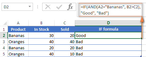
For more IF / AND formula examples, please check out his tutorial: Excel IF function with multiple AND conditions.
An Excel formula for the BETWEEN condition
If you need to create a between formula in Excel that picks all values between the given two values, a common approach is to use the IF function with AND in the logical test.
For example, you have 3 values in columns A, B and C and you want to know if a value in column A falls between B and C values. To make such a formula, all it takes is the IF function with nested AND and a couple of comparison operators:
Formula to check if X is between Y and Z, inclusive:
=IF(AND(A2>=B2,A2<=C2),"Yes", "No")
Formula to check if X is between Y and Z, not inclusive:
=IF(AND(A2>B2, A2<C2),"Yes", "No")
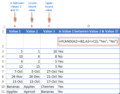
As demonstrated in the screenshot above, the formula works perfectly for all data types - numbers, dates and text values. When comparing text values, the formula checks them character-by-character in the alphabetic order. For example, it states that Apples in not between Apricot and Bananas because the second "p" in Apples comes before "r" in Apricot. Please see Using Excel comparison operators with text values for more details.
As you see, the IF /AND formula is simple, fast and almost universal. I say "almost" because it does not cover one scenario. The above formula implies that a value in column B is smaller than in column C, i.e. column B always contains the lower bound value and C - the upper bound value. This is the reason why the formula returns "No" for row 6, where A6 has 12, B6 - 15 and C6 - 3 as well as for row 8 where A8 is 24-Nov, B8 is 26-Dec and C8 is 21-Oct.
But what if you want your between formula to work correctly regardless of where the lower-bound and upper-bound values reside? In this case, use the Excel MEDIAN function that returns the median of the given numbers (i.e. the number in the middle of a set of numbers).
So, if you replace AND in the logical test of the IF function with MEDIAN, the formula will go like:
=IF(A2=MEDIAN(A2:C2),"Yes","No")
And you will get the following results:
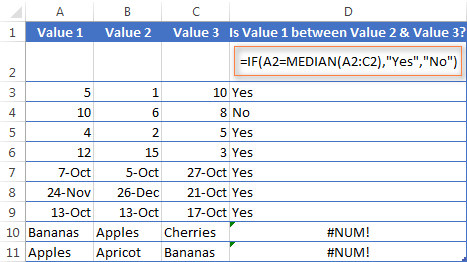
As you see, the MEDIAN function works perfectly for numbers and dates, but returns the #NUM! error for text values. Alas, no one is perfect : )
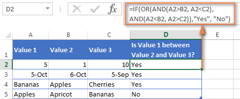
If you want a perfect Between formula that works for text values as well as for numbers and dates, then you will have to construct a more complex logical text using the AND / OR functions, like this:
=IF(OR(AND(A2>B2, A2<C2), AND(A2<B2, A2>C2)), "Yes", "No")
Using the OR function in Excel
As well as AND, the Excel OR function is a basic logical function that is used to compare two values or statements. The difference is that the OR function returns TRUE if at least one if the arguments evaluates to TRUE, and returns FALSE if all arguments are FALSE. The OR function is available in all versions of Excel 2016 - 2000.
The syntax of the Excel OR function is very similar to AND:
Where logical is something you want to test that can be either TRUE or FALSE. The first logical is required, additional conditions (up to 255 in modern Excel versions) are optional.
And now, let's write down a few formulas for you to get a feel how the OR function in Excel works.
| Formula | Description |
=OR(A2="Bananas", A2="Oranges") |
Returns TRUE if A2 contains "Bananas" or "Oranges", FALSE otherwise. |
=OR(B2>=40, C2>=20) |
Returns TRUE if B2 is greater than or equal to 40 or C2 is greater than or equal to 20, FALSE otherwise. |
=OR(B2=" ", C2="") |
Returns TRUE if either B2 or C2 is blank or both, FALSE otherwise. |

As well as Excel AND function, OR is widely used to expand the usefulness of other Excel functions that perform logical tests, e.g. the IF function. Here are just a couple of examples:
IF function with nested OR
=IF(OR(B2>30, C2>20), "Good", "Bad")
The formula returns "Good" if a number in cell B3 is greater than 30 or the number in C2 is greater than 20, "Bad" otherwise.
Excel AND / OR functions in one formula
Naturally, nothing prevents you from using both functions, AND & OR, in a single formula if your business logic requires this. There can be infinite variations of such formulas that boil down to the following basic patterns:
=AND(OR(Cond1, Cond2), Cond3)
=AND(OR(Cond1, Cond2), OR(Cond3, Cond4)
=OR(AND(Cond1, Cond2), Cond3)
=OR(AND(Cond1,Cond2), AND(Cond3,Cond4))
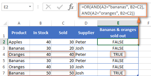
For example, if you wanted to know what consignments of bananas and oranges are sold out, i.e. "In stock" number (column B) is equal to the "Sold" number (column C), the following OR/AND formula could quickly show this to you:
=OR(AND(A2="bananas", B2=C2), AND(A2="oranges", B2=C2))
OR function in Excel conditional formatting
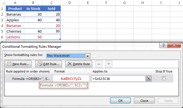
=OR($B2="", $C2="")
The rule with the above OR formula highlights rows that contain an empty cell either in column B or C, or in both.
For more information about conditional formatting formulas, please see the following articles:
Using the XOR function in Excel
In Excel 2013, Microsoft introduced the XOR function, which is a logical Exclusive OR function. This term is definitely familiar to those of you who have some knowledge of any programming language or computer science in general. For those who don't, the concept of 'Exclusive Or' may be a bit difficult to grasp at first, but hopefully the below explanation illustrated with formula examples will help.
The syntax of the XOR function is identical to OR's :
The first logical statement (Logical 1) is required, additional logical values are optional. You can test up to 254 conditions in one formula, and these can be logical values, arrays, or references that evaluate to either TRUE or FALSE.
In the simplest version, an XOR formula contains just 2 logical statements and returns:
- TRUE if either argument evaluates to TRUE.
- FALSE if both arguments are TRUE or neither is TRUE.
This might be easier to understand from the formula examples:
| Formula | Result | Description |
=XOR(1>0, 2<1) |
TRUE | Returns TRUE because the 1st argument is TRUE and the 2nd argument is FALSE. |
=XOR(1<0, 2<1) |
FALSE | Returns FALSE because both arguments are FALSE. |
=XOR(1>0, 2>1) |
FALSE | Returns FALSE because both arguments are TRUE. |
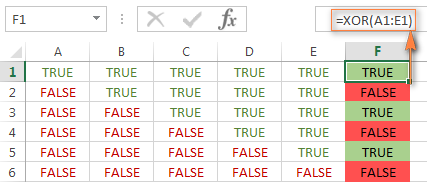
When more logical statements are added, the XOR function in Excel results in:
- TRUE if an odd number of the arguments evaluate to TRUE;
- FALSE if is the total number of TRUE statements is even, or if all statements are FALSE.
The screenshot below illustrates the point:
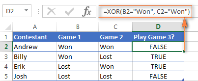
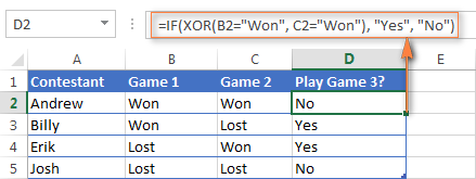
If you are not sure how the Excel XOR function can be applied to a real-life scenario, consider the following example. Suppose you have a table of contestants and their results for the first 2 games. You want to know which of the payers shall play the 3rd game based on the following conditions:
- Contestants who won Game 1 and Game 2 advance to the next round automatically and don't have to play Game 3.
- Contestants who lost both first games are knocked out and don't play Game 3 either.
- Contestants who won either Game 1 or Game 2 shall play Game 3 to determine who goes into the next round and who doesn't.
A simple XOR formula works exactly as we want:
=XOR(B2="Won", C2="Won")
And if you nest this XOR function into the logical test of the IF formula, you will get even more sensible results:
=IF(XOR(B2="Won", C2="Won"), "Yes", "No")
Using the NOT function in Excel
The NOT function is one of the simplest Excel functions in terms of syntax:
You use the NOT function in Excel to reverse a value of its argument. In other words, if logical evaluates to FALSE, the NOT function returns TRUE and vice versa. For example, both of the below formulas return FALSE:
=NOT(TRUE)
=NOT(2*2=4)
Why would one want to get such ridiculous results? In some cases, you might be more interested to know when a certain condition isn't met than when it is. For example, when reviewing a list of attire, you may want to exclude some color that does not suit you. I'm not particularly fond of black, so I go ahead with this formula:
=NOT(C2="black")
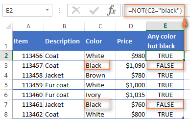
As usual, in Microsoft Excel there is more than one way to do something, and you can achieve the same result by using the Not equal to operator: =C2<>"black".
If you want to test several conditions in a single formula, you can use NOT in conjunctions with the AND or OR function. For example, if you wanted to exclude black and white colors, the formula would go like:
=NOT(OR(C2="black", C2="white"))
And if you'd rather not have a black coat, while a black jacket or a back fur coat may be considered, you should use NOT in combination with the Excel AND function:
=NOT(AND(C2="black", B2="coat"))
Another common use of the NOT function in Excel is to reverse the behavior of some other function. For instance, you can combine NOT and ISBLANK functions to create the ISNOTBLANK formula that Microsoft Excel lacks.
As you know, the formula =ISBLANK(A2) returns TRUE of if the cell A2 is blank. The NOT function can reverse this result to FALSE: =NOT(ISBLANK(A2))
And then, you can take a step further and create a nested IF statement with the NOT / ISBLANK functions for a real-life task:
=IF(NOT(ISBLANK(C2)), C2*0.15, "No bonus :(")
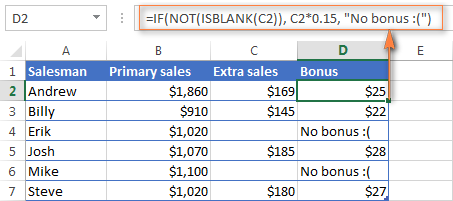
Translated into plain English, the formula tells Excel to do the following. If the cell C2 is not empty, multiply the number in C2 by 0.15, which gives the 15% bonus to each salesman who has made any extra sales. If C2 is blank, the text "No bonus :(" appears.
In essence, this is how you use the logical functions in Excel. Of course, these examples have only scratched the surface of AND, OR, XOR and NOT capabilities. Knowing the basics, you can now extend your knowledge by tackling your real tasks and writing smart elaborate formulas for your worksheets.
 by
by
564 comments
Hello,
I am trying to write a formula that would return a value in cell H3.
I want to divide cell H14 by H24
If that value is greater than 100%, I want it to return 100%
If that value is less that 100%, I want it to return the true value of H14 divided by H24
Thank you for your help.
Hi! I have already given you the formula. If you want to calculate percentages in this formula, use these instructions: How to calculate percentage in Excel - formula examples.
Hi, Please could you help with the below formula?
I have the last training taken date in column BO and calculated the number of months to till date in column BP by using this formula (=IFERROR(($BK$1-BO3)*12/365,"Not Applicable") - Here BK indicates the cut-off date and BO indicates last training date. If an employee was not part of any program the BO column will show "not applicable"
Now I would like to calculate eligibility for a training program based on the number of months since the last training program. Between 6-12 months of the previous training program, an employee is eligible to take another training. Below is the formula that I've tried but is not working.
=IF(OR(BO3="Not Applicable","Eligible",IF(OR(BP3=6, "Eligible","Not Eligible"))
Appreciate your help. Thanks!
Hi! I’m sorry, but your description doesn’t give me a complete understanding of your task. Therefore, I can't offer you a formula. However, you are not using the OR function correctly to write the conditions. I recommend that you read these guidelines: Excel IF OR statement with formula examples.
Help Needed:
I require a row to fill red if the following 2 criteria are met:
1) Cell in column "N" Doesn't contain the word "Collected" (Cells in this column are drop down lists with 9 text options to pick from)
2) Cell in column "M" on the same row has a date older then today "<TODAY()"
How do i combine these into a formula conditional formatting will understand.
Thank you.
Hi! If I understand your task correctly, the following conditional formatting formula should work for you:
=AND(ISNUMBER(SEARCH("Collected",N1)),M1How to find substring in Excel
Hello Alexander
Thank you for the assistance
=AND(ISNUMBER(SEARCH("Collected",$N1)),$M1) highlights all rows containing "collected" and doesn't seem to be taking dates into account.
To clarify, column "M" contains dates as dd/mm/yy
I require a formula to highlight a row when ANYTHING OTHER THAN "Collected" is written in the "N" column cell and the "M" cell on the same row has a date older then todays date.
thank you for the assistance, it is very appreciated.
Hello! I'm sorry, the formula is incomplete:
=AND(ISNUMBER(SEARCH("Collected",N1)),M1<TODAY())
Hope this is what you need.
Hi there,
I have found this to be super helpful so far and was finally able to create an OR formula!
However, I am trying to figure out if it is possible to change the colour of a cell if it is TRUE (checkbox) but there must also be a value in the rest of the row and if there isn't the colour of the cell doesn't change or remains false.
I currently have 2 conditions set which work to a degree.
The conditions I have currently are
1. Value is equal to TRUE - which makes the cell green which means we have ordered something.
2. Custom formula is OR(H17>0,I17>0,J17>0) which turns the cell with the checkbox yellow if there are any values over 0 in the 17 row. This just means we know which rows we need to tick off as ordered.
This works in that when I enter values into the 17th row then the cell with the tick-box changes to yellow so I know what I need to tick off as ordered, and then when I finally tick it off it turns green.
The only time this doesn't work is when someone accidentally presses the checkbox when there are no values in the rest of the row as the cell still changes to green so I am trying to make it that the box cannot be ticked (preferably) or cannot turn green unless there is also a value in the 17th row.
I hope this makes sense.
Hi! Unfortunately, this information is not enough to give you any advice. I can't guess which cell the checkbox is in. It is also unknown what rule is used for the green color. Maybe this guide will be helpful: Excel IF statement for blanks and non-blanks. Or provide additional details to highlight exactly what you need.
Hi, I would like to check if the value in a single cell matches any of the values in a number of other cells. Is there a way to identify those other cells as a set so that the value in the cell to be checked need only be referenced once. That is, if I want to check if cell A1 is equal to any of cells B1, B2 or B3, I can achieve this with IF(OR(A1=B1,A1=B2,A1=B3)), but I would like something like IF(A1=SOMESETFUNCTION(B1:B3))
thanks!
Roger
Hi! To identify duplicates, you can use the COUNTIF function. For example:
=IF(=COUNTIF(B1:B10,A1),"duplicates","")
You can see this and other ways in this article: How to find duplicates in Excel.
I have 6 drop down options in B2, and 3 drop down options in C2 that would give a value for C3. I currently have this =IF(C2="Plate", "$50.00","$45.00"),
But would like something that would include something like, =IF(and)(B2="10U")(C2="Plate", "$50.00"), for all drop down option combinations in B2 & C2. Any help would be great.
Hi! Since you have many conditions, I recommend using the IFS function with the AND operator. For example:
IFS(AND(B2="10U",C2="Plate"), "$50.00", .....)
Want to add colors to a list of number in relation to their total average. The numbers will change every month which means the average will change. How do I assign colors to the numbers? What function or formula should I use.
10
20
30
40
50
60
70
average is 40
how do i use the average (40) to asgin colors - white, yellow, red, green and blue. White the highest and blue the lowest
Hi!
If I understand correctly, try using color scales. The following tutorial should help: How to make a heat map in Excel. I hope my advice will help you solve your task.
Dear Alexander,
If I have the following in cells A1 to A4, is there a formula to check the first 3 characters of any city and also the last 2 numbers of the city and if the number of the city is odd then return abc and if even return xyz
Paris10
London11
Toronto12
Madrid13
Thank you in advance.
Hello!
Get the last two digits with the RIGHT function. Use the MOD function with a divisor of 2 to determine an odd number. The remainder of the division will be equal to 1.
Please use the following formula
=IF(MOD(RIGHT(A2,2),2),"abc","xyz")
Thank you very much for your reply.
In cell A5 I will be repeating the city again, so I would like the formula to look at if it is Paris, London or Toronto and if it is Paris always return abc or xyz based on the even or odd numbers, if it is London then return def or ghi and so on for each different city.
Basically, detect the city and return different value based on the last two numbers of the city being odd or even.
Hi!
You would save me time if you explained the whole task at once.
Column H - Paris, London .....
Column G - abc, .....
Column I - xyz, .....
=IF(MOD(RIGHT(A2,2),2), INDEX(H1:H5,MATCH(TRUE,ISNUMBER(SEARCH(G1:G5,A2)),0)), INDEX(I1:I5,MATCH(TRUE,ISNUMBER(SEARCH(G1:G5,A2)),0)))
Hope this is what you need.
Thank you for your reply. It did not work.
would like the formula to look at if it is Paris, London or Toronto and if it is Paris always return abc or xyz based on the even or odd numbers, if it is London then return def or ghi and so on for each different city when repeated.
Paris10 abc
Paris11 xyz
London10 def
London11 ghi
Paris13 xyz
London17 ghi
Paris10 abc
Hi!
The formula works. Formulate your questions accurately and in detail. If you need abc for even values, swap columns G and I.
Column I - abc, def.....
Column G - xyz, ghi.....
I have 2022 YR (52 week Sale data) and i am current working in 4 week of 2023. How can we calculate average of previous 26 week when i put week number (2023 week) in Cell No. "B2".
Please suggest
Hi!
I'm sorry, I'm afraid these pieces of info are not enough to give you a formula.
What does "week number (2023 week)" mean?
Try to use instruction Excel AVERAGEIF function to average cells with condition, or give a detailed description of the problem.
how can you get the formula of all the students?
I have a drop down list of Cash, Transfer & Cheque in D11 and I want the value in E11 to repeat on E19 whenever I choose "cash" from the drop down list in D11 and also I want "cash" to automatically appear on D19 at the same time, So can anyone tell me how do I make it happen or which formula should I be looking for to make it happen ?
Hello!
Use the IF function in cell D19:
IF(D11="cash",E11,"")
Hi,
Please help to write a formula as per below Logic in Excel.
I want to first check a cell for any data, then want to use if formula with multiple condition with AND funtion
Dear Sir,
Thank you for the great excel topics.
I have a question and hope to find a solution for it. I have 5 columns with the following contents "Large" - "Medium" - "Small", I would like to use the majority as the desired results; for example, column1 = Large, column2 = Large, column3 = Large, column4 = Medium, column5 = small, then I would recommend the desired results will be "Large" as it represents the majority of the contents.
How to solve this problem? And develop a function that can apply to these issues to a more extensive set of cells. I have a large dataset, and I need to use this rule. How?
I appreciate any help you can provide.
Ali
Hello!
MATCH function returns the position of each value. MODE function determines which position occurs most frequently. INDEX function returns the value at this position.
Please check the formula below, it should work for you:
=INDEX(A1:A10,MODE(MATCH(A1:A10,A1:A10,0)))
I need to put a condition, if any three or more than three columns out of 15 columns satisfy a certain condition I need to get it as true.
Please help me out.
Hi!
Turn a logical expression into a number using a mathematical operation. Use the SUM formula to count TRUE values.
For example,
=IF((SUM(--(A2:O2>7)))>=3,TRUE)
Hello, i have a formula that i am trying to use =COUNTIFS('Master Data'!D:D,UTC!E2,'Master Data'!B:B,"01",'Master Data'!M:M,"O-Open",'Master Data'!K:K,"AIPR",'Master Data'!K:K,"ANSM",'Master Data'!K:K,"AWNM",'Master Data'!K:K,"AWSM",'Master Data'!K:K,"CAWI") however, the issue with this formula is that i need it to guarantee that it matches ('Master Data'!D:D,UTC!E2,'Master Data'!B:B,"01",'Master Data'!M:M,"O-Open",'Master and meets some of 'Master Data'!K:K,"AIPR",'Master Data'!K:K,"ANSM",'Master Data'!K:K,"AWNM",'Master Data'!K:K,"AWSM",'Master Data'!K:K,"CAWI") criteria. I'm not too familiar with logic or AND, OR functions could someone please assist?
Hi!
It is very difficult to understand a formula that contains unique references to your workbook worksheets. I can't figure out what match you want to get. Hence, I cannot check its work, sorry.
Please describe your problem in more detail.
sorry I made a mistake in the last msg.
Hello!
I am in school right now learning accountant and business start up but I am having a little bit of trouble with some parts of excel functions. I learned some parts quickly and some others just do not want to sink in my brain. Can anyone help/explain to me how I would come to this answer. Please. details of how to come to the answer would be helpful . I am a visual person.
Example:
When a property is sold, the agent receives a commission based on the category of the building. For a commercial building, a commission rate of 4% is applied, otherwise, 3% is applied. Write down the arguments of the IF formula that you will enter in cell D5 to determine the commission received for the first entry.
A B C D
4-- ENTRY CATEGORY SELLING PRICE COMMISSION
5-- 07-QC4002 Residential $ 240,000
6-- 07-QC4005 Commercial $ 410,000
7-- 07-QC4006 Investment $ 536,000
=IF(__________________________,______________________________,_____________________________)
Hi!
You can find the examples and detailed instructions here: Using IF function in Excel: formula examples.
i need a formulae which can help me asign diffrent numbers that add up to the whole number i have in a cell.
Data compersated Gift Bundle
15 300 mbs
500 mbs
1 GB
1.5GB
3 GB
5 GB
For example breaking down 15 in to the diffrent bundles to add up to 15
Hi!
Unfortunately, your problem cannot be solved using formulas. An Excel formula can only insert a value into the cell in which it is written.
SL. No Name Math Science English Total RESULT
1 VIMAL AB 66 34 100
2 SANJAY 79 53 77 209
3 GUDU 44 21 59 124
4 SAROHI 38 45 23 106
5 TARUN 68 AB 56 124
6 RAMAN 25 53 46 124
7 AKASH 49 75 47 171
8 DIPU 73 61 AB 134
9 MANOJ 57 32 55 144
10 MANJU 76 54 61 191
what is the results
AB=absent , so its fail, all subject attened is pass
Hi!
Sorry, it's not quite clear what you are trying to achieve.
I need formula for calculation of marks results with different grades, (if candidate fail any one subject it should be shows fail like that IF formula)
Hi, I have produced a vlookup table which gives two variables, one column being being glazing type and other column being orientation (n,s,e,w) which then give a value based on the combination of these two variables.
What formula do i need to use?
There are three variables in the first column and 4 variables in the second column and depending which combination of these are selected they correspond to a given value in column 3.
In the main spreadsheet i have columns a and b as drop down menus to select the appropriate glazing type and orientation. Column c in the main spreadsheet is where i wish to input the formula to dispaly the corresponding value
Hello!
If I understood the problem correctly, you need to do a vlookup based on two criteria. I recommend paying attention to this article.
I hope my advice will help you solve your task.
Hi,
I'm trying to create a pointing system in which I have 3 types & 3 categories (both are columns):
For example: Types are:
Black
Brown
Yellow
Categories are columns with value (duration).
1 year
2 years
3 years
I can't create a formula that will create a result like the below:
If black & 1 year then return value 1$
If black & 2 years then return value 2$
If black & 3 years then return value 3$
If brown & 1 year then return value 3$
If brown & 2 yers then return value 4$
And so on:
How can I do this?
Hi!
You didn’t provide enough data to suggest a formula. Are the values of some cells compared to types and categories? Not all conditions are listed. I recommend paying attention to the nested IF functions or the IFS function.
I want write formula like this. I have a drop down list of a,b,c . If i select a , value will 2, If i select b,value will 3 and if select c ,value will be 3 . It will be multiply with another value 20. How to write this formula
Hi!
The drop-down list writes a value from this list to the cell.
hi all
I beg for assistance,if I had 20000KSH of my basic salary and I was given 10% for the house allowance from the basic salary.Use logical function to carry out this.
I WOULD LIKE YOU TO OPEN FOR ME FULL SPACE SO THAT I CAN TRY TO CARRY OUT SOME LOGICAL FUNCTIONS IN EXCEL
Please correct below formula
=COUNTIFS('Design Status'!$C$7:$C$68,Sheet1!B12)*(AND(C13>='Design Status'!I7:I68))
Can i share the record