This tutorial explains how to use MATCH function in Excel with formula examples. It also shows how to improve your lookup formulas by a making dynamic formula with VLOOKUP and MATCH.
In Microsoft Excel, there are many different lookup/reference functions that can help you find a certain value in a range of cells, and MATCH is one of them. Basically, it identifies a relative position of an item in a range of cells. However, the MATCH function can do much more than its pure essence.
Excel MATCH function - syntax and uses
The MATCH function in Excel searches for a specified value in a range of cells, and returns the relative position of that value.
The syntax for the MATCH function is as follows:
Lookup_value (required) - the value you want to find. It can be a numeric, text or logical value as well as a cell reference.
Lookup_array (required) - the range of cells to search in.
Match_type (optional) - defines the match type. It can be one of these values: 1, 0, -1. The match_type argument set to 0 returns only the exact match, while the other two types allow for approximate match.
- 1 or omitted (default) - approximate match (closest smaller). Finds the largest value in the lookup array that is less than or equal to the lookup value. Requires sorting the lookup array in ascending order, from smallest to largest or from A to Z.
- 0 - exact match. Finds the first value in the array that is exactly equal to the lookup value. No sorting is required.
- -1 - approximate match (closest larger). Finds the smallest value that is greater than or equal to the lookup value. The lookup array should be sorted in descending order, from largest to smallest or from Z to A.
To better understand the MATCH function, let's make a simple formula based on this data: students names in column A and their exam scores in column B, sorted from largest to smallest. To find out where a specific student (say, Laura) stands among others, use this simple formula:
=MATCH("Laura", A2:A8, 0)
Optionally, you can put the lookup value in some cell (E1 in this example) and reference that cell in your Excel Match formula:
=MATCH(E1, A2:A8, 0)
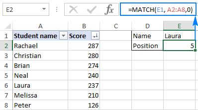
As you see in the screenshot above, the student names are entered in an arbitrary order, and therefore we set the match_type argument to 0 (exact match), because only this match type does not require sorting values in the lookup array. Technically, the Match formula returns the relative position of Laura in the range. But because the scores are sorted from largest to smallest, it also tells us that Laura has the 5th best score among all students.
Tip. In Excel 365 and Excel 2021, you can use the XMATCH function, which is a modern and more powerful successor of MATCH.
4 things you should know about MATCH function
As you have just seen, using MATCH in Excel is easy. However, as is the case with nearly any other function, there are a few specificities that you should be aware of:
- The MATCH function returns the relative position of the lookup value in the array, not the value itself.
- MATCH is case-insensitive, meaning it does not distinguish between lowercase and uppercase characters when dealing with text values.
- If the lookup array contains several occurrences of the lookup value, the position of the first value is returned.
- If the lookup value is not found in the lookup array, the #N/A error is returned.
How to use MATCH in Excel - formula examples
Now that you know the basic uses of the Excel MATCH function, let's discuss a few more formula examples that go beyond the basics.
Partial match with wildcards
Like many other functions, MATCH understands the following wildcard characters:
- Question mark (?) - replaces any single character
- Asterisk (*) - replaces any sequence of characters
Note. Wildcards can only be used in Match formulas with match_type set to 0.
A Match formula with wildcards comes useful in situations when you want to match not the entire text string, but only some characters or some part of the string. To illustrate the point, consider the following example.
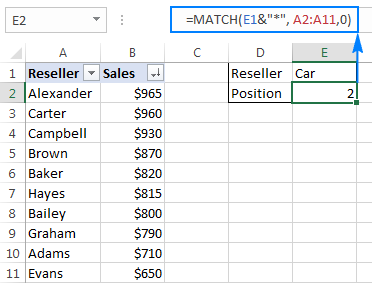
Supposing you have a list of regional resellers and their sales figures for the past month. You want to find a relative position of a certain reseller in the list (sorted by the Sales amounts in descending order) but you cannot remember his name exactly, though you do remember a few first characters.
Assuming the reseller names are in the range A2:A11, and you are searching for the name that begins with "car", the formula goes as follows:
=MATCH("car*", A2:A11,0)
To make our Match formula more versatile, you can type the lookup value in some cell (E1 in this example), and concatenate that cell with the wildcard character, like this:
=MATCH(E1&"*", A2:A11,0)
As shown in the screenshot below, the formula returns 2, which is the position of "Carter":
To replace just one character in the lookup value, use the "?" wildcard operator, like this:
=MATCH("ba?er", A2:A11,0)
The above formula will match the name "Baker" and rerun its relative position, which is 5.
Case-sensitive MATCH formula
As mentioned in the beginning of this tutorial, the MATCH function doesn't distinguish uppercase and lowercase characters. To make a case-sensitive Match formula, use MATCH in combination with the EXACT function that compares cells exactly, including the character case.
Here's the generic case-sensitive formula to match data:
The formula works with the following logic:
- The EXACT function compares the lookup value with each element of the lookup array. If the compared cells are exactly equal, the function returns TRUE, FALSE otherwise.
- And then, the MATCH function compares TRUE (which is its lookup_value ) with each value in the array returned by EXACT, and returns the position of the first match.
Please bear in mind that it's an array formula that requires pressing Ctrl + Shift + Enter to be completed correctly.
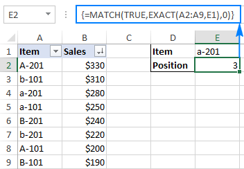
Assuming your lookup value is in cell E1 and the lookup array is A2:A9, the formula is as follows:
=MATCH(TRUE, EXACT(A2:A9,E1),0)
The following screenshot shows the case-sensitive Match formula in Excel:
Compare 2 columns for matches and differences (ISNA MATCH)
Checking two lists for matches and differences is one of the most common tasks in Excel, and it can be done in a variety of ways. An ISNA/MATCH formula is one of them:
For any value of List 2 that is not present in List 1, the formula returns "Not in List 1". And here's how:
- The MATCH function searches for a value from List 1 within List 2. If a value is found, it returns its relative position, #N/A error otherwise.
- The ISNA function in Excel does only one thing - checks for #N/A errors (meaning "not available"). If a given value is an #N/A error, the function returns TRUE, FALSE otherwise. In our case, TRUE means that a value from List 1 is not found within List 2 (i.e. an #N/A error is returned by MATCH).
- Because it may be very confusing for your users to see TRUE for values that do not appear in List 1, you wrap the IF function around ISNA to display "Not in List 1" instead, or whatever text you want.
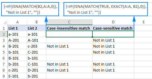
For example, to compare values in column B against values in column A, the formula takes the following shape (where B2 is the topmost cell):
=IF(ISNA(MATCH(B2,A:A,0)), "Not in List 1", "")
As you remember, the MATCH function in Excel is case-insensitive by itself. To get it to distinguish the character case, embed the EXACT function in the lookup_array argument, and remember to press Ctrl + Shift + Enter to complete this array formula:
=IF(ISNA(MATCH(TRUE, EXACT(A:A, B2),0)), "Not in List 1", "")
The following screenshot shows both formulas in action:
To learn other ways to compare two lists in Excel, please see the following tutorial: How to compare 2 columns in Excel.
Excel VLOOKUP and MATCH
This example assumes you already have some basic knowledge of Excel VLOOKUP function. And if you do, chances are that you've run into its numerous limitations (the detailed overview of which can be found in Why Excel VLOOKUP is not working) and are looking for a more robust alternative.
One of the most annoying drawbacks of VLOOKUP is that it stops working after inserting or deleting a column within a lookup table. This happens because VLOOKUP pulls a matching value based on the number of the return column that you specify (index number). Because the index number is "hard-coded" in the formula, Excel is unable to adjust it when a new column(s) is added to or deleted from the table.
The Excel MATCH function deals with a relative position of a lookup value, which makes it a perfect fit for the col_index_num argument of VLOOKUP. In other words, instead of specifying the return column as a static number, you use MATCH to get the current position of that column.
To make things easier to understand, let's use the table with students' exam scores again (similar to the one we used at the beginning of this tutorial), but this time we will be retrieving the real score and not its relative position.
Assuming the lookup value is in cell F1, the table array is $A$1:$C$2 (it's a good practice to lock it using absolute cell references if you plan to copy the formula to other cells), the formula goes as follows:
=VLOOKUP(F1, $A$1:$C$8, 3, FALSE)
The 3rd argument (col_index_num) is set to 3 because the Math Score that we want to pull is the 3rd column in the table. As you can see in the screenshot below, this regular Vlookup formula works well:
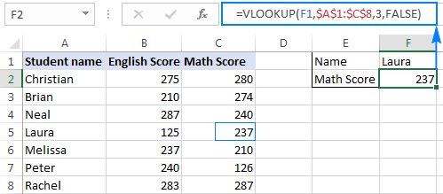
But only until you insert or delete a column(s):
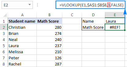
So, why the #REF! error? Because col_index_num set to 3 tells Excel to get a value from the third column, whereas now there are only 2 columns in the table array.
To prevent such things from happening, you can make your Vlookup formula more dynamic by including the following Match function:
MATCH(E2,A1:C1,0)
Where:
- E2 is the lookup value, which is exactly equal to the name of the return column, i.e. the column from which you want to pull a value (Math Score in this example).
- A1:C1 is the lookup array containing the table headers.
And now, include this Match function in the col_index_num argument of your Vlookup formula, like this:
=VLOOKUP(F1,$A$1:$C$8, MATCH(E2,$A$1:$C$1, 0), FALSE)
And make sure it works impeccably no matter how many columns you add or delete:
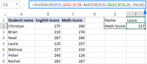
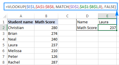
In the screenshot above, I locked all cell references for the formula to work correctly even if my users move it to another place in the worksheet. A you can see in the screenshot below, the formula works just fine after deleting a column; furthermore Excel is smart enough to properly adjust absolute references in this case:
Excel HLOOKUP and MATCH
In a similar manner, you can use the Excel MATCH function to improve your HLOOKUP formulas. The general principle is essentially the same as in case of Vlookup: you use the Match function to get the relative position of the return column, and supply that number to the row_index_num argument of your Hlookup formula.
Supposing the lookup value is in cell B5, table array is B1:H3, the name of the return row (lookup value for MATCH) is in cell A6 and row headers are A1:A3, the complete formula is as follows:
=HLOOKUP(B5, B1:H3, MATCH(A6, A1:A3, 0), FALSE)

As you have just seen, the combination of Hlookup/Vlookup & Match is certainly an improvement over regular Hlookup and Vlookup formulas. However, the MATCH function doesn't eliminate all their limitations. In particular, a Vlookup Match formula still cannot look at its left, and Hlookup Match fails to search in any row other than the topmost one.
To overcome the above (and a few other) limitations, consider using a combination of INDEX MATCH, which provides a really powerful and versatile way to do lookup in Excel, superior to Vlookup and Hlookup in many respects. The detailed guidance and formula examples can be found in INDEX & MATCH in Excel - a better alternative to VLOOKUP.
This is how you use MATCH formulas in Excel. Hopefully, the examples discussed in this tutorial will prove helpful in your work. I thank you for reading and hope to see you on our blog next week!
Practice workbook for download
Excel MATCH formula examples (.xlsx file)
 by
by
84 comments
Hi,
Need match formula help....I'm currently using the formula =MATCH(a2,c:c,FALSE) and instead of #N/A in the cell I want it to enter a symbol. Is this possible?
Hi! To replace an error message with a symbol or word, use the IFERROR function. Read more: How to use IFERROR in Excel with formula examples.
hi, I have multiple tab spreadsheet. One tab has the master list of addresses each tab represents a region. Column A has letter in each region that matches an entry on the master list. I want to use the information in from the master list column B and C to popuate columns B and C on the region tabs Any direction would be greatly appreciated
I am using Match(A1&B1,$D:$D,0) to produce the row no of that item in Col D, My problem is that the function gives the answer 0 in all cases. I can prove that there are cases when $A1 & B$1 do equal a value in D. I can find no reference to the meaning of 0 as an answer to Match. The answer #N/A is when there is no match
Hi! I can't check your formula because I don't have your data.
Hello - I'm looking to use index/match in a rank formula, but it's not quite working the way I need it to. My current formula is:
RANK(E3,INDEX(E:E,0,MATCH((F3=F:F)*(A3=A:A),0)))
E3 --> is the cell I need to rank from values in column E
BUT I don't want to rank all of the cells in column E, just a subset of the full list
So I decided to use Index/Match to just pull the subset of column E cells I want to rank against:
F3 and A3 are my keys to this subset (they're a name and number that occur multiple times in the sheet)
But my formula just brings back the entire column E in the rank equation; my index/match do not narrow it down at all!
Open to all and any help! thanks
Hi! The MATCH function can return only a single position number. Also, the RANK function cannot determine the relative position of a number separately in a group of values. I recommend using this instruction: How to rank in Excel by group.
I believe the following formula will help you solve your task:
=SUMPRODUCT((F3=F:F)*(A3=A:A)*(E3<E:E))+1
Wonderful! Thank you Alexander
HELLO SIR,
I HAVE A PROBLEM.
MY PROBLEM IS-
order-id SKU order-id
112-3195379-9870667 112-3195379-9870667 0 FORMULA -=INDEX($V$3:$V$2605,MATCH(W604,$H$3:$H$2605,0))
112-3195379-9870667 Pharma436528461 112-3195379-9870667 0
112-3195379-9870667 Pharma436528461 112-3195379-9870667 0
112-3195379-9870667 Pharma436528461 112-3195379-9870667 0
112-3195379-9870667 Pharma436528461 112-3195379-9870667 0
112-3195379-9870667 Pharma436528461 112-3195379-9870667 0
I NEED SKU VALUE BUT IT IS TAKING BLANK VALUE, PLEASE HELP
Your formula contains no errors. Check the data you are looking for. I cannot help here.
I want to create a match formula where the lookup data is in another sheet.
For example, I want to look or match the amount of 4,407.72 in Sheet called "Look", row 7
The look up value in the tab called "Data" starting from row B1 to B3. I am using the integer function with match to avoid small differences.
4,407.72
4,507.00
4,508.00
My formula array on c9 is not working. It wont even let me complete the formula array. From the data, is should see row with a value of 4407.72, since, the integer value of it is 4,407.72.
=MATCH(C7,data!INT(B1:B3),0)
Any help would be much appreciated.
Hi! The integer value 4407.72 is 4407. Read the INT function manual carefully. Only an integer can be searched among other integers. Perhaps the formula will look like this:
MATCH(INT(C7),data!INT(B1:B3),0)
I have two Sheet one with column A has a first and last name ( Nael Odeh) and Sheet two has a column A has a full name (Nael Ahmad Mustafa Odeh)
how I can right a match statement for these two columns
Hi!
I don't know exactly how you want to compare text values. However, I think these instructions will be helpful: Excel IF statement for partial text match
Hello, I am having an issue with the match formula. The cell referenced to the lookup_value is in a date format, but it is searching it as number format, giving me N/A.
Hello!
Dates in Excel are stored as numbers. Note that the data you're looking for a date in is also dates, not text. I hope this helps, or give more details.
Hi Alex!
Quick and silly question:
I have a row with accumulative net income for every month (- 400K , -250K, -70K, 89K, ....etc)
How do I get the month where accumulative net income turns positive? ( For the example I'm giving the answer of course should be 4).
Hello!
To find the position of the first positive value, use the MATCH formula:
=MATCH(TRUE,A1:A10>0,0)
I hope it’ll be helpful.
Hi, thank you for your post. I have multiple column and for each I want to retrieve the first or the last column not empty. With match I need to insert an argument: do you have any advice?
Best regards
Luca
Hello!
To find in column the last cell with a number -
=MATCH(1E+300,A1:A1000,1)
To find the last cell containing text -
=MATCH(REPT("z",100),A1:A1000,1)
To find the last non-empty cell, use ISBLANK function -
=MAX(ROW(A1:A1000)*NOT(ISBLANK(A1:A1000)))
Hope this is what you need.
I have report dates as headers in multiple columns, which are not on any particular interval. I need to calculate the aging between Two Report Dates (old report date to latest report date) if the cell value matches to my criteria. I am looking to solve a recruitment problem here. Where, I have all the different Recruitment statuses as each row item. Example : on 1st August if a particular candidate HR status matches to interview and on 7th August also if the status is same as Interview. Then, i need to calculate the aging for this particular candidate. if HR status on 7th August is not an interview, then I shouldn't calculate the aging there. this loop has to continue until the status gets updated. which means if the candidate is in the same status as Interview on 25th August report date. then I need to calculate the aging between 1st august to 25th august.
which means, I need to calculate aging from the date when the candidate first hit the interview stage till the time he is in the same stage.
thanks in advance.
Hello!
Try to use the recommendations described in this article: Calculate difference between two dates in days, weeks, months or years.
I hope it’ll be helpful.
i have a list of dates in ascending order in Col A and wish to find the first and last date row of each month and i am using the formulae MATCH(C2,$A:$A,1). However for the first day of the month i am getting erratic rows. Can you please help.
Date Match Date Row
01/01/2022 01/01/2022 3
01/01/2022 01/02/2022 7
03/01/2022 01/03/2022 9
28/01/2022 01/04/2022 17
01/02/2022
01/02/2022 31/01/2022 5
03/02/2022 28/02/2022 9
28/02/2022 31/03/2022 14
03/03/2022 30/04/2022 19
03/03/2022
04/03/2022
05/03/2022
30/03/2022
01/04/2022
01/04/2022
01/04/2022
02/04/2022
05/04/2022
Hi!
Use the EOMONTH function to determine the first and last day of the current month.
To find the row number with the first date of the month from cell A1, use the formula
=IFERROR(MATCH(EOMONTH(A1,-1),$A$1:$A$10,1)+1,1)
To find the row number with the last date of the month, try the formula
=MATCH(EOMONTH(A1,0),$A$1:$A$10,1)
If this is not what you wanted, please describe the problem in more detail.
Hi,
A have a list of team names as the columns (B1, C1, D1 etc, etc). Under each team is a list of dates which relates to dates of matches they have.
Column A is the match number each date is for each team. (A2 is 1, A3 is 2, A4 is 3 etc, etc)
ie, 30th Jul 22 may be match 1 for one team but match 3 for another.
In another sheet I have the team name and the date but I want to be able to find which match number it is.
Can this be done please?
Hello!
Here is the article that may be helpful to you: INDEX MATCH MATCH and other formulas for two-way lookup.
Here is an example of the formula:
=INDEX(Sheet2!A2:A4, MATCH(Sheet1!B1,INDEX(Sheet2!B2:E4,, MATCH(Sheet1!A1,Sheet2!B1:E1,0)),0))
A1 - team. B1 - date
I hope my advice will help you solve your task.
Perfect, thank you very much for the help.
Alex,
I have a match formula that I would like to return blank if there is nothing to return. Can you give advice on this one. Example, as you know a formula that reads, " =IF(ISERROR(MATCH($A2,'[WORKBOOK_2.xlms]Tab-1'!$A$2:$A$200,0)),"NO","YES")" will return a No or yes depending if there is a match or not. And will continue to display a "no" when there is nothing in the cell.
My question is, how do I return nothing or return a blank cell if there is no values in a range of cells yet?
Hello!
Use the nested IF function and the ISBLANK function to check a range of blank cells.
For example:
=IF(SUM(--NOT(ISBLANK(A2:A200)))=0,"", IF(ISERROR(MATCH($A2,'[WORKBOOK_2.xlms]Tab-1′!$A$2:$A$200,0)),”NO”,”YES”) )
I hope my advice will help you solve your task.
Hello There,
First of all, can't thank you guys for being so helpful in improving excel use in our day to day job. Many thanks.
I am looking for numbers from one sheet in another sheet, which is quite easy, but the problem is that I want to check the integer of numbers both in source and destination. This formula does not help:
=MATCH(INT(H4),INT('[AllReport.xlsx]Sheet1'!$F$3931:$F$6846),0)
any advise?
Kind regards
Hello!
This formula includes an external reference. It will only work if this file is opened in Excel.
I recommend reading this guide: Excel reference to another sheet or workbook (external reference).
Hi,
You guys are amazing with your quick support and I hope you can help me solving the problem that gives me sleepless nights. I’m trying to figure out the formula that refers to the value in a different sheet and counts automatically the total number of that specific value on a specific date.
Let’s say Sheet1 has in column A time stamps with Date and Time, in column B it contains info about Scheduled Appt and indicates if it’s either a Direct buyer or from a Broker. Now in Sheet2 the cell A1 has the date that column A from Sheet1 should match with. The cell B1 from Sheet2 has the value that should be counted from column B in Sheet1 and the total should be displayed in B2 in Sheet2. I don’t know what I’m doing wrong, but it keeps giving me error messages. I tried to list below how it looks in Excel to make it easier to understand, I hope it's displayed correctly:
Sheet 1
A B C
1 Scheduled Appt Walk-In
2 5/21/2022 1:02:45 Direct Broker
3 5/21/2022 4:22:13 Direct Direct
4 5/21/2022 18:22:13 Broker Broker
Sheet 2
A B C
1 5/21/2022 Direct Broker
2 Scheduled Appt
3 Walk-In
Thank you so much in advance for your help!
Hello!
If I understand your task correctly, the following formula SUMPRODUCT should work for you:
=SUMPRODUCT(--(INT(Sheet1!A2:A4)=Sheet2!$A$1),--(Sheet1!B2:B4=Sheet2!$B$1))
Hope this is what you need.
i want
A B C D
1 a
1 b
2 a
1 c
2 b
3 a
in this case, i want column A match and sub-branch in B column and in b column match only one came value should be get "0" get multiple result get in B column get should be "1"
Hi!
I am not sure I fully understand what you mean.
sir,
I Need In column A has sum numbers and B column has some Letters in this case I need for example 1 number is repeated 3 times in Column A, and column B having Deferent value more then one, in this case, I want result "1" and number 3 is having only one value in this case I want to get "0"
Hi!
Based on your description, it is hard to completely understand your task. However, I’ll try to guess and offer you the following formula:
=COUNTIF($B$1:B1,B1)
Copy this formula down along the column.
You can learn more about COUNTIF function in Excel in this article on our blog.
i need to look up for a date (exact match) in a column and the value available in the next row in that column.
please suggest the formla
Hello!
I recommend reading this guide: How to use INDEX MATCH in Excel.
Please try the following formula:
=INDEX(A1:A20,MATCH(D1,A1:A20,0)+1)
I am trying to write a formula that finds the last matching data in a cell and calculate the time between the two. ex column A is dates, column B are things (A,B,C & D), column C is the amount of days between the last time "D" was entered.
4/1/2021 C
4/3/2021 A
4/5/2021 D
4/6/2021 D 1 days
4/12/2021 C 11 days
4/20/2021 D 14 days
Thanks
Hello!
If I understand your task correctly, write the formula in cell C2
=IFERROR(A2-LOOKUP(2, 1/($B$1:$B1=B2), $A$1:$A1),"")
After that you can copy this formula down along the column.
Please check out this article to learn how to get a value associated with the last entry in a row.
Match function did help half the purpose as I needed the 'position' it last appeared.
However, I tried and it can only be applicable to one column of appearance.
With multiple column of appearances to how to get the last position
For Example:
A B C D E F
1 1 2 3 4 5 6
2 2 3 7 8 9 10
3 1 3 4 8 9 10
I used =Match (A1, A2:A3, 0) ................ yes it will return 2, which is OK.
But I tried ...
=Match (B1, A2:F3, 0) .............................. It will give me an error instead of 1, which is the answer.
As the match function seems to comb vertical and single column. Can it look up both ways (vertically and horizontally across multiple columns) and still return the last row position?
Thank you.
Hello!
To find the line number in which the last required value is located (cell I1), you can use the formula:
=MAX(IF($A$2:$G$7=$I$1,ROW($A$2:$A$7),0))
I hope this will help, otherwise please do not hesitate to contact me anytime.
I dont understand. In the above set data shown there are not G column, and what is cell I8?
Your answer maybe referring to the wrong question
Hi,
Mistake. Instead of I8, read I1. The formula returns the last row number that contains the value from I1.
If this is not what you need, explain the problem in more detail.
Formula =Match(A1, A2:A3, 0) return error, not 2.
=Match(B1, A2:F3, 0) return 2, not error.
Maybe instead of Match(B1, A2:F3, 0)
try
=MAX(IF($A$2:$F$3=$B$1,ROW($A$2:$A$3),0))
Hi Alexander,
Thanks for the reply. The first column of numbers is actually the excel mandatory numbers
A B C D E F
1 1 2 3 4 5 6
2 2 3 7 8 9 10
3 1 3 4 8 9 10
I used =Match (A1, A2:A3, 0) ................ yes it will return 2, which is OK.
But I tried ...
=Match (B1, A2:F3, 0) .............................. It will give me an error instead of 1, which is the answer. As it is the last position it last occur. 1 row down.
I tried your formula, but still got an error. Have you tried it in excel?
Thanks!!!!!
=IFNA((MATCH(A1,A2:A3,0)),0)&IFNA((MATCH(A1,B2:B3,0)),)&IFNA((MATCH(A1,C2:C3,0)),)&IFNA((MATCH(A1,D2:D3,0)),)&IFNA((MATCH(A1,E2:E3,0)),)&IFNA((MATCH(A1,F2:F3,0)),)
Found the formula that i want. I wonder if there is a shorter version.
Thanks Alexander.
but the formula is wrong... is the table extends out with repetitive numbers. sigh
Hi,
The formula works. It is a pity that you did not manage to apply it.
How do i apply it? It returns an error.
Hi
I am trying to find the first time a specific amount or number is found (equal or higher than the value I am looking for) above or below in the same column.
Match works for looking down in the column, but not up - unless I am missing something here.
Any ideas?
Hello!
If I understand your task correctly, the following formula should work for you:
=INDEX($A$2:$A$8,MATCH(MIN(IF((($A$2:$A$8>=A2)*(ROW($A$2:$A$8)<>ROW(A2)))>0,$A$2:$A$8-A2)),IF((($A$2:$A$8>=A2)*(ROW($A$2:$A$8)<>ROW(A2)))>0,$A$2:$A$8-A2),0))
I hope my advice will help you solve your task.
Hi folks! Great article. I need help please -
Scenario - I have 12 columns dated Jan to Dec with cumulative totals under each column. E.g.
Jan - 5000
Feb - 10000
March - 20,000
April - 45,000
May - 90,000
and so on.
I have another column that provides me with a total number. E.g.
Total Funding Amount = 50,000
I need to create another column, called month of funding breach that can add the cumulative total from the months above by matching it to the total funding amount, and return a string i.e the month. E.g. Since total funding amount is 50,000, funding will run out in May. I need this month to be populated in the new column 'Funding Breach Month.'
Can anyone assist please?
Hello Geetha!
Do you want to determine the month in which the running total amount is greater than the total amount of funding?
If the total funding amount are calculated on row 30, then use the formula
=VLOOKUP((MATCH(50000,A30:L30,1)+1), {1,"January";2,"February";3,"March";4,"April";5,"May";6,"June";7,"July"; 8,"August";9,"September";10,"October";11,"November";12,"December"},2,0)
Hope this is what you need.
I I am trying to match the first 4 digits in the column to the first 4 digits in another column and if there's a match I want the value associated with the column. My code keep saying #NA: =INDEX(Sheet1!$B$2:$B$100, MATCH(LEFT($F2,3), Sheet1!$B$2:$B$100,1))
Hello Melissa!
Your formula is looking for the first 3 (not 4) characters from cell F3 in column B. Moreover, in column B, the formula is not looking for the first 3 characters, but looking for text of 3 characters. The search failed, so an N/A error appears. I do not know what data you are using, so I can not say the cause of the error.
Maybe this formula will work
=INDEX($B$2:$B$100, MATCH(LEFT($F2,3), LEFT($B$2:$B$100,3),0))
Great explanation! Thank you.
Hi
Is there a way to list all matches for one search criteria? For example, if on sheet 1 I have Column A - date, Col B - number, Col C - name.
Is there a way on Sheet 2, to have a search criteria where the name is entered in D1 (for example), then a formula next to it that lists all the sheet 1 (Column B) numbers that are found each time the name in sheet 2 D1 is matched in sheet 1 Col C?
I have a table that has values being returned by formulas. When I tried MATCH to find the location of a number, it looks for the value in the formulas and can't find anything. Is there a way to tell MATCH to look up in the values, not the formulas? Thanks.
I need to search a data base of guest names who stay at the Hotel in 2018 compared to 2019. how do I search so Excel alerts me to the same name or mobile number appearing twice.
Thank you
I have a large workbook with multiple tabs that all feed each other. Everything that is being fed into other sheets is currently done by linking to individual cells, which means that sorting does not work well. I'm looking for a solution that would allow me to use a unique identifier for each line item, feed info between sheets, and allow the individual sheets to all be sorted without affecting the data presented. Is this possible with INDEX/MATCH?
I am trying to find a better formula to look for a value using index and match. could you please help me to figure out the problem in the below formula. I am not getting the result. the result is "#N/A"
1. {=INDEX(BQ:BQ,MATCH(1,(VLOOKUP(LEFT(BF2,4),BL:BL,1,FALSE))*(BO:BO=D3),0))}
2. {=INDEX(BQ:BQ,MATCH(1,BL:BL=OR(BD2,BE2,BF2))*(BO:BO=D4),0)}
3. {=INDEX(BQ:BQ,MATCH(1,BL:BL=BH2&"*")*(BO:BO=D5),0)}
whereas below formula with single cell reference works fine..
4. {=INDEX(BQ:BQ,MATCH(1,(BL:BL=BC2)*(BO:BO=D6),0))}
Please help.
I am trying to run an index that will look for a specific name in four different columns and if that name appears in any of those columns (or all of them), give me the info that is in the first column.
To do this, the match doesn't seem to work. Is there an or component that can used?
I don't seem be able to use match when the values in the row being searched for a match are in TIME format. I'm trying to find the element that equals "11:38 PM", which is there, but my match formula returns #N/A, I think for a reason related to this. =MATCH("11:38 PM",A2:A12,0). That range does contain the time value. It must be something about indicating the value being sought.
if the same values are there in the both the values then i have to give condition like as "name" so please explain how to do it?
thanks
ramesh
I have a slightly different problem which doesn't seem to be solved by Match because Match will only return the first value. I have a number of surveys done by a number of people on a series of days. Some people will have done the survey more than twice. How can I determine the date difference between each survey and the preceding one, please? When I apply match, index and datedif, only the difference between the latest and the first survey dates is returned. Any suggestions?
Hello,
For me to understand the problem better, please send me a small sample workbook with your source data and the result you expect to get to support@ablebits.com. Please don't worry if you have confidential information there, we never disclose the data we get from our customers and delete it as soon as the problem is resolved.
Please also don't forget to include the link to this comment into your email.
I'll look into your task and try to help.
I have a problem where I need to extract a list of dates between 2 given dates from a vertical array of dates in ascending order. Is this possible using the index match functionality without resorting to VB. I'd rather avoid have blank entries at the top of the generated list too.
Hello, Chris,
supposing that you have the dates in A1:A24, the first given date - in B1 and the second - in B2, you can try the formula similar to the one below, but please keep in mind that it's an array formula and it should be entered by pressing Ctrl+Shift+Enter on your keyboard:
{=IF(SUM(($A$1:$A$24*(A1>$B$1))*($A$1:$A$24*(A1<$B$2)))=0,"",A1)}I kindly ask you to alter it according to the way your data is stored.
If you still have some problems or the formula doesn't work, please send us the workbook with your data to support@ablebits.com . Don't forget to link this comment in your email.
We'll look into your task and try to help.
Unless I am misunderstanding, I think the first example is wrongly explained. Match finds Laura in position 4 because she is the fourth item in the range being searched, not because that is her score ranking as stated. As it happens, she is fifth highest score, not fourth, after Rachael(1st with 287), Christian (2nd with 280), Brian (3rd with 274), Neal (4th - 240). But that's just chance as Match is not looking at the scores, only the names (the A2-A8 range). There is no "offset" to tell it to look at the scores.
In effect, unless you wanted to know where a student's name was positioned in a random list of names, I don't believe this example tells you anything else by itself?
Hi Paul,
That is a good catch! Yes, Match returns Laura's position in the range being searched. And because the scores are sorted from largest to smallest, it is also her position among other students.
For some reason, in my original screenshot, the highest score (Rachael's) appeared at the bottom of the list. Not sure how that could happen, maybe I added it after sorting the Score column. Anyway, I've resorted the column and updated the screenshot. Now, the Match formula returns the 5th position, exactly as it should. I've also added this explanation to the post to make the example clearer.
Thank you again for your feedback!
7/13/2017 1301311 ESI NDT 0936 PIT 2A - NMY 2A SARNO, L. #VALUE! 07/13/2017 A001301311 NTX 9035
by colum 1264012 - A0001264012 how to match - 0
by colum 1264012 - A0001264012
Wow!!
Hello,
I understand all of this very well, when lookup_array is a 1-dimensional array.
But, what if lookup_array is a 2-dimensional array?
Will MATCH return a couple of numbers, representing row and columns?
Thank you,
stefano
Hello, Stefano,
no, MATCH will not return the numbers for both row and column. But depending on your task, you can try another way - use MATCH with INDEX.
Thankful! to you.
Very useful and perfect.
Useful, very detailed explanation, thanks a lot!
Really impressive; I'm really curious about the huge world of excel formulas. I hope I'll learn some of them. You are doing a great job with writing blogs like this.. everyone who wants to learn excel (especially excel formulas) will be thankful for this.
Brilliant work- Am sharing this link to everyone.
Your are good. Your presentation is so awesome. Thanks a lot.
i have table with daily entry
c column to add 1 when A1 is 14 or less, in same time if A1 more than 14
d column give 1
the problem is A1 is increasing every day and i don't want column C to give me zero when A1 more than 14
thank you for help.