This tutorial explains the Excel SUMIF function in plain English. The main focus is on real-life formula examples with all kinds of criteria including text, numbers, dates, wildcards, blanks and non-blanks.
Microsoft Excel has a handful of functions to summarize large data sets for reports and analyses. One of the most useful functions that can help you make sense of an incomprehensible set of diverse data is SUMIF. Instead of adding up all numbers in a range, it lets you sum only those values that meet your criteria.
So, whenever your task requires conditional sum in Excel, the SUMIF function is what you need. A good thing is that the function is available in all versions, from Excel 2000 through Excel 365. Another great thing is that once you've learned SUMIF, it will take you very little effort to master other "IF" functions such as SUMIFS, COUNTIF, COUNTIFS, AVERAGEIF, etc.
SUMIF in Excel - syntax and basic uses
The SUMIF function, also known as Excel conditional sum, is used to add up cell values based on a certain condition.
The function is available in Excel 365, Excel 2021, Excel 2019, Excel 2016, Excel 2013, Excel 2010, Excel 2007, and lower.
The syntax is as follows:
As you see, the SUMIF function has 3 arguments - first 2 are required and the last one is optional.
- Range (required) - the range of cells to be evaluated by criteria.
- Criteria (required) - the condition that must be met. It may be supplied in the form of a number, text, date, logical expression, a cell reference, or another Excel function. For example, you can enter the criteria such as "5", "cherries", "10/25/2014", "<5", etc.
- Sum_range (optional) - the range to sum if the condition is met. If omitted, then range is summed.
Note. Please pay attention that any text criteria or criteria containing logical operators must be enclosed in double quotation marks, e.g. "apples", ">10". Cell references should be used without the quotation marks, otherwise they would be treated as text strings.
Basic SUMIF formula
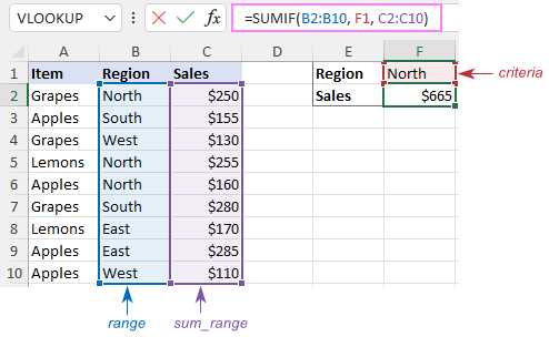
To better understand the SUMIF syntax, consider the following example. Suppose you have a list of products in column A, regions in column B, and sales amounts in column C. Your goal is to get a total of sales for a specific region, say North. To have it done, let's build an Excel SUMIF formula in its simplest form.
You start with defining the following arguments:
- Range - a list of regions (B2:B10).
- Criteria - "North" or a cell containing the region of interest (F1).
- Sum_range - the sales amounts to be added up (C2:C10).
Putting the arguments together, we get the following formula:
=SUMIF(B2:B10, "north", C2:C10)
or
=SUMIF(B2:B10, F1, C2:C10)
Both formulas only sum sales in the North region:
Note. The sum_range parameter actually defines only the upper leftmost cell of the range to be summed. The remaining area is defined by the dimensions of the range argument. In practice, this means that sum_range argument does not necessarily have to be of the same size as range argument, i. e. it may have a different number of rows and columns. However, the top left cell must always be the right one. For example, in the above formula, you can supply C2, or C2:C4, or even C2:C100 as the sum_range argument, and the result will still be correct. However, the best practice is to provide equally sized range and sum_range.
Note. The SUMIF function is case-insensitive by nature. However, it is possible to force it to recognize the text case. For full details, please see Case-sensitive SUMIF in Excel.
How to use SUMIF in Excel - formula examples
Hopefully, the above example has helped you gain some basic understanding of how the function works. Below you will find a few more formulas that demonstrate how to use SUMIF in Excel with various criteria.
SUMIF greater than or less than
To sum numbers greater than or less than a particular value, configure the SUMIF criteria with one of the following logical operators:
- Greater than (>)
- Greater than or equal to (>=)
- Less than (<)
- Less than or equal to (<=)
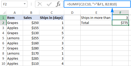
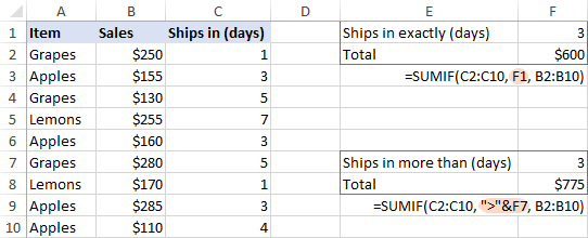
In the table below, supposing you wish to add up the sales numbers for the items that ship in 3 or more days. To express this condition, put a comparison operator (>) before the number and surround the construction in double quotes:
=SUMIF(C2:C10, ">3", B2:B10)
If the target number is in another cell, say F1, concatenate the logical operator and cell reference:
=SUMIF(C2:C10, ">"&F1, B2:B10)
In a similar manner, you can sum values smaller than a given number. For this, use the less than (<) operator:
=SUMIF(C2:C10, "<3", B2:B10)
SUM IF equal to
A SUMIF formula with the "equal to" criteria works for both numbers and text. In such criteria, the equals sign is not actually required.
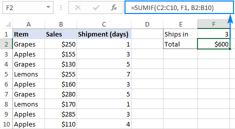
For instance, to find a total of the items that ship in 3 days, either of the below formulas will do:
=SUMIF(C2:C10, 3, B2:B10)
or
=SUMIF(C2:C10, "=3", B2:B10)
To sum if equal to cell, supply a cell reference for criteria:
=SUMIF(C2:C10, F1, B2:B10)
Where B2:B10 are the amounts, C2:C10 is the shipment duration, and F1 is the desired delivery time.
Likewise, you can use the "equal to" criteria with text values. For instance, to add up the Apples amounts, choose any of the formulas below:
=SUMIF(A2:A10, "apples", B2:B10)
=SUMIF(A2:A10, "=apples", B2:B10)
=SUMIF(A2:A10, F1, B2:B10)
Where A2:A10 is the list of items to compare against the value in F1.
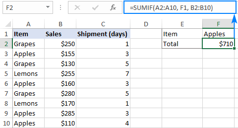
The above formulas imply that the criterion matches the entire cell contents. Consequently, the SUMIF function will add up Apples sales but not, say, Green Apples. To sum partial matches, construct the "if cell contains" criteria like in this SUMIF wildcard formula.
Note. Please pay attention that, in Excel SUMIF formulas, a comparison or equals operator should always be enclosed in double quotes, whether used on its own or together with a number or text.
SUM IF not equal to
To build the "not equal to" criteria, use the "<>" logical operator.
When a value, either text or number, is hardcoded in the criteria, remember to surround the entire construction with double quotes.
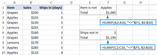
For example, to sum the amounts with shipment other than 3 days, the formula goes as follows:
=SUMIF(C2:C10, "<>3", B2:B10)
To find a total of all the items except Apples, the formula is:
=SUMIF(A2:A10, "<>apples", B2:B10)
When the criterion is in another cell, concatenate the "not equal to" operator and a cell reference like this:
=SUMIF(A2:A10, "<>"&F1, B2:B10)
SUM IF blank
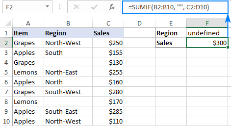
This example shows how to sum cells in one column if a corresponding cell in another column is blank. There are two formulas to fulfill the task. Which one to use depends on your interpretation of a "blank cell".
If "blank" means cells that contain absolutely nothing (no formula, no zero-length string returned by some other function), then use "=" for criteria. For example:
=SUMIF(B2:B10, "=", C2:D10)
If "blank" includes empty strings (for example, cells with a formula like =""), then use "" for criteria:
=SUMIF(B2:B10, "", C2:D10)
Both formulas return a total of sales for undefined regions, i.e. where a cell in column B is blank:
SUM IF not blank
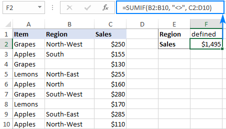
To make "if cell is not blank then sum" kind of formula, use "<>" as the criteria. This will add up all cells that contain anything in them, including zero-length strings.
For instance, here's how you can sum sales for all the regions, i.e. where column B is not blank:
=SUMIF(B2:B10, "<>", C2:D10)
Excel SUMIF with text criteria
When adding up numbers in one column based on text values in another column, it's important to differentiate between exact and partial match.
| Criteria | Formula Example | Description |
|---|---|---|
| Sum if equal to | Exact match: =SUMIF(A2:A8, "bananas", C2:C8) |
Sum values in cells C2:C8 if a cell in column A in the same row contains exactly the word "bananas" and no other words or characters. Cells containing "green bananas", "bananas green", or "bananas!" are not included. |
| Sum if cell contains | Partial match: =SUMIF(A2:A8, "*bananas*", C2:C8) |
Sum values in cells C2:C8 if a corresponding cell in column A contains the word "bananas", alone or in combination with any other words. Cells containing "green bananas", "bananas green", or "bananas!" are summed. |
| Sum if not equal to | Exact match: =SUMIF(A2:A8, "<>bananas", C2:C8) |
Sum values in cells C2:C8 if a cell in column A contains any value other than "bananas". If a cell contains "bananas" together with some other words or characters like "yellow bananas" or "bananas yellow", such cells are summed. |
| Sum if cell does not contain | Partial match: =SUMIF(A2:A8, "<>*bananas*", C2:C8) |
Sum values in cells C2:C8 if a cell in column A does not contain the word "bananas", alone or in combination with any other words. Cells containing "yellow bananas" or "bananas yellow" are not summed. |
For real-life formula examples, please check out Sum if equal to and Sum if not equal to.
In the next section, we'll take a closer look at SUMIF formulas with partial match.
SUMIF formulas with wildcard characters
To conditionally sum cells by partial match, include one of the following wildcard characters in your criteria:
- Question mark (?) to match any single character in a specific position.
- Asterisk (*) to match any number of characters.
Example 1. Sum values based on partial match
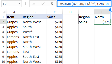
Suppose you wish to total sales for all northern regions, including North, North-East, and North-West. To have it done, put an asterisk right after the word "north":
=SUMIF(B2:B10, "north*", C2:D10)
An asterisk on both sides will also work:
=SUMIF(B2:B10, "*north*", C2:D10)
Alternatively, you can type the region of interest in a predefined cell (F1), and then concatenate a cell reference and a wildcard character enclosed in quotes:
=SUMIF(B2:B10, F1&"*", C2:D10)
Or
=SUMIF(B2:B10, "*"&F1&"*", C2:D10)
Example 2. Sum if cell contains * or ?
To match a literal question mark or asterisk, place a tilde (~) before the character, e.g. "~?" or "~*".
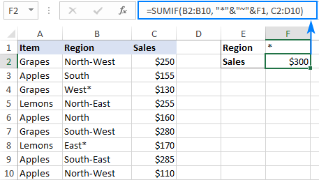
For example, to sum sales for the regions marked with *, use "*~*" for criteria. In this case, the first asterisk is a wildcard and the second one is a literal asterisk character:
=SUMIF(B2:B10, "*~*", C2:D10)
If the criteria (* in our case) is entered in a separate cell, then concatenate a tilde and the cell reference, like this:
=SUMIF(B2:B10, "*"&"~"&F1, C2:D10)
Example 3. Sum if another cell contains text
If your dataset contains various data types and you only want to sum cells corresponding to text values, the following SUMIF formulas will come in handy.
To add up values in cells C2:C8 if a cell in column A contains any text character(s):
=SUMIF(A2:A8,"?*", C2:C8)
To sum values in C2:C8 if a cell in column A contains any text value, including zero length strings:
=SUMIF(A2:A8,"*", C2:C8)
Both of the above formulas ignore non-text values such as numbers, dates, errors, and Booleans.
How to use Excel SUMIF with dates
Using dates as SUMIF criteria is very much like using numbers. The most important thing is to supply a date in the format that Excel understands. If you are not sure which date format is supported and which is not, the DATE function can be a solution.
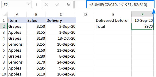
Assuming you are looking to sum sales for the items delivered before 10-Sep-2020, the criteria can be expressed in this way:
=SUMIF(C2:C10, "<9/10/2020", B2:B10)
or
=SUMIF(C2:C10, "<"&DATE(2020,9,10), B2:B10)
or
=SUMIF(C2:C10, "<"&F1, B2:B10)
Where F1 is the target date.
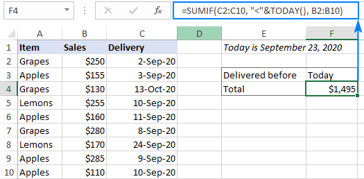
To sum cells based on today's date, include the TODAY function in your criteria. For example, that's how you calculate a total of sales with a delivery date prior to today:
=SUMIF(C2:C10, "<"&TODAY(), B2:B10)
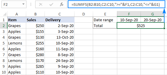
To sum within a date range, you need to define a smaller and larger date separately. This can be done with the help of the SUMIFS function that supports multiple criteria.
For example, to sum values in column B if a date in column C is between two dates, this is the formula to use:
=SUMIFS(B2:B10, C2:C10, ">="&F1, C2:C10, "<="&G1)
Where B2:B10 is the sum range, C2:C10 is the list of dates to check, F1 is the start date and G1 is the end date.
More formula examples can be found in SUMIFS with date range as criteria.
How to do SUMIF from another sheet
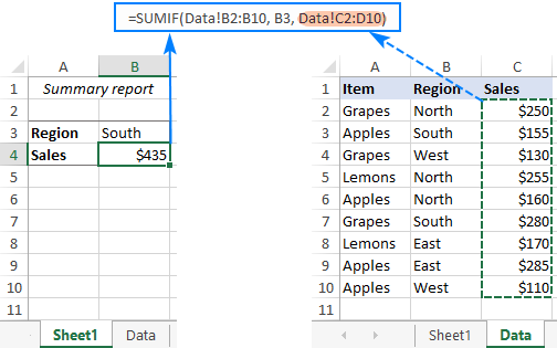
To conditionally sum data from a different sheet, provide external references for the SUMIF arguments. The easiest way is to start typing a formula, switch to another worksheet and select ranges using the mouse. Excel will insert all the references automatically, without you having to worry about the correct syntax.
For instance, the below formula will add up values in C2:C10 on the Data sheet based on the criteria in B3 on Sheet1:
=SUMIF(Data!B2:B10, B3, Data!C2:C10)
How to correctly use cell references in SUMIF criteria
To create a flexible formula, you normally insert all variable parameters in predefined cells instead of "hardcoding" them. With Excel SUMIF, that might be a bit of a challenge.
In the simplest case when summing "if equal to", you simply use a cell reference for criteria. For example:
=SUMIF(C2:C10, F1, B2:B10)
But when a cell reference is used together with a logical operator, the criteria should be provided in the form of a string. So, you use the double quotes ("") to start a text string and ampersand (&) to concatenate and finish the string off. For example:
=SUMIF(C2:C10, ">"&F7, B2:B10)
Please note that the comparison operators are enclosed in quotation marks while the cell references are not.
Why is my SUMIF formula not working?
There could be several reasons why Excel SUMIF is not working for you. Sometimes, your formula does not return what you expect only because the data type in a cell or in some argument isn't suited for the SUMIF function. Below is a list of important things to check.
1. SUMIF supports only one condition
The syntax of the SUMIF function has room for only one condition. To sum with multiple criteria, either use the SUMIFS function (adds up cells that meet all the conditions) or build a SUMIF formula with multiple OR criteria (sums cells that meet any of the conditions).
2. Range and sum_range should be of the same size
For a SUMIF formula to work correctly, the range and sum_range argument should have the same dimensions, otherwise you may get misleading results. The point is that Microsoft Excel does not rely on the user's ability to provide matching ranges, and to avoid possible inconsistency issues, it determines the sum range automatically in this way:
Sum_range defines only the upper left cell of the range that will be summed, the remaining area is determined by the size and shape of the range argument.
Given the above, the below formula will actually sum cells in C2:C10 and not in C2:D10. Why? Because range consists of 1 column and 9 rows, and so does sum_range.
=SUMIF(B2:B10, "north", C2:D10)
In older Excel versions, unequally sized ranges can cause lots of problems. In modern Excel, complex SUMIF formulas where sum_range has less rows and/or columns than range are also capricious. That is why it's a good practice to always define the same number of rows and columns for these two arguments.
3. Range and sum_range should be ranges, not arrays
Though SUMIF can process an array constant in criteria like shown in this example, it does not support arrays in range and sum_range. These two arguments can only be cell ranges.
5. SUMIF criteria syntax
For criteria, the SUMIF function allows using different data types including text, numbers, dates, cell references, logical operators (>, <, =, <>), wildcard characters (?, *, ~) and other functions. The syntax of such criteria is quite specific.
If the criteria argument includes a text value, wildcard character or logical operator followed by text, number or date, enclose the whole criteria in quotation marks. For example:
=SUMIF(B2:B10, "north*", C2:D10)
=SUMIF(C2:D10, ">100")
=SUMIF(B2:B10, "<>north", C2:D10)
=SUMIF(C2:C10, "<=9/10/2020", B2:B10)
When a logical operator is followed by a cell reference or another function, the criteria should be provided in the form of a string. So, you use an ampersand (&) to concatenate a logical operator and a reference or function. For example:
=SUMIF(B2:B10, ">"&F1)
=SUMIF(C2:D10, "<="&TODAY(), B2:B10)
4. SUMIF from another workbook not working
As with many Excel functions, SUMIF can refer to other sheets and workbooks, provided they are currently open.
For example, this formula will work fine as long as Book1 is open:
=SUMIF([Book1.xlsx]Sheet1!$A$2:$A$9,"apples",[Book1.xlsx]Sheet1!$F$2:$F$9)
And it will stop working as soon as Book1 is closed. This happens because the referenced ranges in closed workbooks get de-referenced into arrays. And since arrays are not supported in the range and sum_range arguments, SUMIF throws a #VALUE! error.
6. SUMIF does not recognize text case
By design, SUMIF in Excel is not case-sensitive, meaning it treats uppercase and lowercase letters as the same characters. To make a case-sensitive SUMIF formula, use the SUMPRODUCT function together with EXACT.
That's how to use SUMIF in Excel. Hopefully, our formula examples have given you some good insights. As always, I thank you for reading and hope to see you on our blog next week!
Practice workbook for download
Excel SUMIF examples (.xlsx file)
 by
by
343 comments
I am hoping someone can help, I am not great with figuring out how to use IF and SUMIF, this is what I came up with, but it's returning a value of TRUE instead of adding the numbers I need. Any suggestions? I'm guessing what I have is way off, I am trying to use a formula from another sheet and customize it to fit what I need.
I am trying to total a range of numbers if the customer name is the same, see table, if A is the same, add the corresponding totals in difference, into cell total. Can anyone help? I'm stumped.
This is what I tried to use =IF($A2="","","IF(($A2=$A3))"",SUMIFS($I$2:$I2,$A$2:$A2,$A2,""")
Helper FullName ItemCode ItemDesc 2024 NetTotal StoreId 2023 Difference Total
, S1000B13 , S1000B SS COAL TAR SLR BULK 655 $3,058.85 13 0 655 TRUE
, S1000B5 , S1000B SS COAL TAR SLR BULK 50 $202.50 5 0 50
, S1000UB13 , S1000UB SS COAL TAR ULTRA BLEND WITH SAND 926 $3,592.23 13 0 926
, S1097UB13 , S1097UB PMM- POLYMER MODIFIED MASTERSEAL ULTRA BLEND WITH SAND 896 $3,727.36 13 0 896
Hi! I am sorry to say that your description of the problem is not clear to me. I can't understand and check your formula because it contains errors and is written incorrectly. What does "add the corresponding sums in difference" mean? To help me understand the problem, please give me an example of the data in column A, data in column I and expected result in each row.
What I'm trying to do is, when cells are identical in column A(Helper) add the numbers in column H, and that formula will be written in column I. Does that make sense?
I misstated that. What I'm trying to do is, when cells are identical in column A(Helper) add the numbers in column I (Difference), and that formula will be written in column J(Total).
Hi! To find sum for the same values in column A, you can use SUMIF function and the recommendations from the article above. But without an example of the data and the result you want, your description is impossible to understand.
Hello,
For some reason, my sumif formula is adding together unique characters together, and I can't seem to figure out why.
My formula is sumif(W:W,Lookupvalue,U:U)
LookupValue Sumif
002058010050331005050011 257,070
002058010050331005252131 257,070
002058010050331006450314 257,070
002058010050331006450316 257,070
Column U Column W
Consolidated Ending Bal Lookup Value
198,469.06 002058010050331005050011
4,624.84 002058010050331005252131
44,546.34 002058010050331006450314
9,430.06 002058010050331006450316
__________
257,070.30
Hi! When the SUMIF function compares Lookup Value to a value in a cell in column W, this value is automatically converted to the number 2.05801005050331E+21. The last 9 digits in column W are ignored and replaced with zeros. Therefore, you will get the same result as if all the cells in the W column had the same value.
To sum values by condition, try the SUMPRODUCT function:
=SUMPRODUCT(U1:U4*(W1:W4=V1))
Hi there,
Thanks so much for the explanation! I added a character at the end of my lookup values and it seemed to have fixed the issue,
I appreciate it
I'm trying to do a =sumif(large for #s in column A based on if column b meets a specific criteria.. I can't seem to get it right...
I hope you have studied the recommendations in the tutorial above. Please clarify your problem or provide additional information to understand what you need.
Hello Geoff
what is wrong in this form?
=SUMIF(B3:B86;""*"&[@[CÀPSULES]]&"*";G3:G86)")
Thank you
Hi! I can't understand your formula and check it as I don't have your data.
Why isn't my SUMIF formula working? This is the formula which isn't working:
=SUMIF(Table16[EEs covering the course or programme (unique identifier)],"*[@[Unique Identifier]]*",Table16[PG ONLY
TOTAL (higher + lower rates / no. EEs)])
It brings back the value 0.
When I replace the table cell reference with a specific string, the formula works:
=SUMIF(Table16[EEs covering the course or programme (unique identifier)],"*smi3*",Table16[PG ONLY
TOTAL (higher + lower rates / no. EEs)])
Hi! If you use a cell reference, add asterisks using the & concatenation operator. Please re-read in this article above - Example 1. Sum values based on partial match.
Instead of "*[@[Unique Identifier]]*" write "*"&[@[Unique Identifier]]&"*"
Hi Alexander, thank you for the help. I've tried each of these versions and none of them works:
=SUMIF(Table16[EEs covering the course or programme (unique identifier)],"*[@[Unique Identifier]]*",Table16[PG ONLYTOTAL (higher + lower rates / no. EEs)])
=SUMIF(Table16[EEs covering the course or programme (unique identifier)],"*"[@[Unique Identifier]]"*",Table16[PG ONLYTOTAL (higher + lower rates / no. EEs)])
=SUMIF(Table16[EEs covering the course or programme (unique identifier)],"*A2*",Table16[PG ONLYTOTAL (higher + lower rates / no. EEs)])
=SUMIF(Table16[EEs covering the course or programme (unique identifier)],"*"A2"*",Table16[PG ONLYTOTAL (higher + lower rates / no. EEs)])
Oh sorry I just noticed the &!
Dear Sir,
how to apply this formula =SUMIFS(D1:D5,B1:B50,E2,C1:C5001,L1) NEXT ROW AND COLUMNS
Hi! In the SUMIFS formula, all criterion ranges must have the same size, as has been written about many times on this blog.
I have 11 digit numeric codes data in column A and amounts in Column B. I want to summarize it on the basis of first 6 Digits of Codes in column A.
I have 11 digit alpha-numeric codes data in column A and amounts in Column B. I want to summarize it at first 6 Digits of Codes in column A.
Hi! You can use the SUMPRODUCT function to find the sum of values based on a partial match of a criterion.
=SUMPRODUCT(--(ISNUMBER(SEARCH($F$1,A1:A10)))*(B1:B10))
F1 - 6 Digits of Code
For more information, please read: How to find substring in Excel
I am trying to build a formula uses cells for the criteria that is part of sumif function. For example.
F20 = '[C2:C23]
F19 = 'A2:A23
c20 = sumif(F19,A22,F20)
Please let me know what I'm doing wrong.
thanks
Don
Hi! Only references to data cells and criterion values can be arguments of the SUMIF function. Read carefully the article above.
On Sheet1 in SmartSheet I have:
- a Project Reference column which could include whole numbers (i.e. 4) to identify Parent projects or decimals (i.e. 4.1, 4.2, 4.3) to identify sub-projects within the parent project. Eventually this project reference column could contain numbers from 1 to 100.
- a Project column which lists the project name and/or any sub-project names as children tasks
- a Total Actuals Sub-Project column which uses the following formula: "=SUMIFS({Sheet2 FY24 YTD}, {Sheet2 Project Ref}, [Project Reference]@row, {Sheet2 Res/Act}, "ACTUALS")"
- a Total Actual per Project column: the formula for this is where I'm having trouble. See explanation further below.
On Sheet2 in SmartSheet I have:
- a Project Reference column (this column is manually updated with the associated project reference assign from Sheet1
- a Reserve/Actual column in which either Reserve or Actuals is selected
- a Project column that uses the following formula to auto-populate the exact project name from Sheet1: "=INDEX({Sheet1 Range 1: Project}, MATCH([Project Reference]@row, {Sheet1 Range 1: Project Ref}, 0))"
- a FY24 YTD column which SUMS designated cells
I'm having trouble creating the formula for Total Actual per Project column on Sheet1. What I'd like it to do is look at the parent row - in this case the Project Reference # is 4, with 4.1, 4.2, 4.3 as sub-projects (it's important to note here that not all projects have sub-projects) - and add the values from Total Actuals Sub-project column IF the value in the Project Reference column is >= 4 AND <=4.999.
Is this possible? Somebody PLEASE help!
Thank you!
Hi! Unfortunately, I could not understand your problem. Try to describe it more shortly, give an example of source data and desired result.
Hello,
I am totalling numbers from column A based on criteria in column B.
But I need the numbers from column A only to be totalled if they are between $25,001 and $50,000. How do i add this condition.
Essentially i need to merge these to formulars.
=SUMIF($K$3:$K$1129,P1,$E$3:$E$1129)
=SUMIFS(E:E,E:E,">"&P24,E:E,"<"&P25)
Hi! Use the SUMIFS function and add all the conditions to this formula. For example:
=SUMIFS($E$3:$E$1129,$K$3:$K$1129,P1,$E$3:$E$1129,">"&P24,$E$3:$E$1129,"<"&P25)
Hello, can we automatically sort column in the criteria without put the criteria one by one into the formula. Example i have 60 criteria that want to sum up, how exactly we can simply sort the criteria without put in the formula one by one.
SUMIF(range, Apple, [sum_range]) , SUMIF(range, Ball, [sum_range]), SUMIF(range, Class, [sum_range])................
How to simplified without put in formula one by one
Hi! If you want to sum values with multiple OR conditions, try this formula:
SUM(SUMIF(range,[criteria range],[sum_range]))
Hi I would like to sum up the following numbers using the "Total Row" in a table. However, I need to keep the "XXK" format due to instructions given , which makes me not able to add up the cells that contain text "K".
10K
10K
8K
8K
8K
10K
0
10K
10K
Any solution for this case? Thanks!
Hi! Replace the letter "K" with "000" using the SUBSTITUTE function. Then turn the text into a number and calculate the sum. Try this formula:
=SUM(--SUBSTITUTE(A1:A8,"K","000"))
Hi,
How to be able use function in the creteria range that contain the symbol ">" ? and how put the creteria?
=SUMIFS($A$4:$A$13,$B$4:$B$13,">61",$C$4:$C$13,"Infinity")
Hi! If I understand your task correctly, try the following formula:
=SUMIFS($A$4:$A$13,$B$4:$B$13,"*>61*",$C$4:$C$13,"Infinity")
The search criterion corresponds to the pattern *>61*, which means that any text that contains the phrase ">61" anywhere in the cell can be found.
Is possible to find sum for number in a cell displayed using if condition?. Example=if(A1=Orange,"104",if(A1=Mango,"105"))
Help please if you are aware about this
Hi! I'm not quite sure what you want to do, but the text in the formula must be enclosed in quotation marks. For example, A1="Orange". You do not need to use quotation marks with numbers.
I'm trying to use (L6,P6)*10 <- this formula, if cell Q6 contains the word yes. Can someone help me with the text for this function?
Hi!
If I understand correctly, use the IF function to calculate by condition.
=IF(Q6="yes",L6*10,"")
(L6,P6)*10 -incorrect.
Value for same criteria e.g., "interest 22-23" is to be collected from 4 sheets of same workbook. How to use SUMIF function for it.
Kindly advise.
Thanks
Hello!
To conditionally sum data from a multiple sheets, use external references for the SUMIF arguments. Pay attention to the following paragraph of the article above: How to do SUMIF from another sheet. Also use recommendations from this article: SUMIF multiple columns with one or several criteria in Excel.
For example:
=SUMIF(Data1!B2:B10, B3, Data1!C2:C10) + SUMIF(Data2!B2:B10, B3, Data2!C2:C10)
When =sum(C70:C75) of a column of numbers derived by =SUMIF($B$6:$B$64,$B70,C$6:C$64) ==> i get zero (0) no matter how I format the number (e.g., general, accounting, currency, etc.) How can I correct this?
I can't see your data, so I can't give advice.
how do i write the formula if the value of the right hand column is over 4 at any time add 1 to the left hand column instead?
Hours Mins
1 1
0 3
1 1
0 3
0 2
2 10
£48.92 £61.16
so it will read 4 and 2 instead of 2 and 10
Thank you
Sorry, it's not quite clear what you are trying to achieve. I don't see the relationship between your question and the supposed result. Please clarify your specific problem or provide additional information to understand what you need.
What is the formula if i want total sum of 1 cell will not exceed 29. The excess will carry over to the next cell if reach the total at 30 ,automatically converted into 1 count which the value carry over.
Thanks
Hi!
To do calculations by condition, use the IF function.
For example:
=IF(SUM(A2:A10)>29,29,SUM(A2:A10))
=IF(SUM(A2:A10)>29,SUM(A2:A10)-29,0)
Hope this is what you need.
i have 10 invoices, want to sum only those invoices whose sum is nearer to certain value. e.g.
Invoice Value Nearest sum required less than or equals to 1000
A-1 100
A-2 350
A-3 240
A-4 370
A-5 400
A-6 110
A-7 50 50
A-8 900
A-9 950 950
A-10 700
from above A-7 & A-9 invoice sum is less than or equals to 1000
please suggest any formula
i have 10 invoices, i want to sum invoices (it may be 1 invoice or multiple) whose sum will be nearest to certain limit. how to do ?
Hi!
You can find the solution to your problem with the Excel Solver add-in. Read more How to use Solver in Excel with examples.
How sum if
A B C
20 30 40
10 50 90
40 60 30
70 30 60
In the above eg. I want a sum of column C from the Min or Max value of column A or B. As A2 has the first occurrence of min/max value so from there I want the sum of the C column (90+30+60) C2 to C4.
I m giving another for better understanding the query
A B C
20 90 30
10 30 40
20 10 50
50 30 50
10 50 20
in this eg. max or min value from column A & column B which appears/comes first is B1 (90). So from B1, I want the sum in column C, from C1 to C5 (30+40+50+50+20)
Please help with this question.
Hello!
To create a reference to a range of cells, use the INDIRECT function. Here is an example of a formula:
=SUM(INDIRECT("C"&MATCH(MIN(A1:A20),A1:A20,0)&":C"&MATCH(9999999,C1:C20,1)))
Hi
I have studied the above, and it works well,
I am stuck on when I need to sum up a weekly column but avoid entering the date range every time.
=SUMIFS('TO PHL FROM UK'!H:H, 'TO PHL FROM UK'!O:O, ">=16/01/2023", 'TO PHL FROM UK'!O:O, "<=22/01/2023")
I would like to be able to drag the formula down so the date range stays 7 days but moves along to 23/1/2023 - 29/1/2023 (UK date format)
please kindly advise
thanks
Hi!
Replace the dates in the formula with relative references to the cells in which the desired values will be written. When you copy a formula, these references will change.
Hi
Can you assist with a formula for me..
if the name in column A (NAME) is the same, add the amounts for that name from column B (BILL) and provide a sum total in column C (TOTAL BILLS)
The first list below is the data, and further below is my expected results
Name Bill TOTAL BILLS
Lewis £100.00
Lewis £150.00
Abby £20.00
Abby £30.00
Abby £50.00
Abby £10.00
Martin £80.00
Martin £105.00
--------------------------------------------------------------------------------------------------------------------------------------------------------
Name Bill TOTAL BILLS
Lewis £100.00 £250.00
Lewis £150.00
Abby £20.00 £110.00
Abby £30.00
Abby £50.00
Abby £10.00
Martin £80.00 £185.00
Martin £105.00
Thanks so much
Hi
I hope you have studied the recommendations in the tutorial above. It contains answers to your question
I have two columns of numbers, A and B. I want to Sum the numbers in column B where the corresponding number in A is not "" (that parts easy) and where the corresponding number in A is greater than the number in B and I want to do this all in a formula in one cell. Is that possible with Summifs using Google Sheets?
Hello Geoff,
Yes, it's possible :) You will find the answers (and examples) in the tutorial devoted to SUMIFS for Google Sheets.