The tutorial shows how to use the TEXTJOIN function to merge text in Excel with practical examples.
Until recently, there were two prevalent methods to merge cell contents in Excel: the concatenation operator and CONCATENATE function. With the introduction of TEXTJOIN, it seems like a more powerful alternative has appeared, which enables you to join text in a more flexible manner including any delimiter in between. But in truth, there's much more to it!
Excel TEXTJOIN function
TEXTJOIN in Excel merges text strings from multiple cells or ranges and separates the combined values with any delimiter that you specify. It can either ignore or include empty cells in the result.
The function is available in Excel for Office 365, Excel 2021, and Excel 2019.
The syntax of the TEXTJOIN function is as follows:
Where:
- Delimiter (required) - is a separator between each text value that you combine. Usually, it is supplied as a text string enclosed in double quotes or a reference to a cell containing a text string. A number supplied as a delimiter is treated as text.
- Ignore_empty (required) - Determines whether to ignore empty cells or not:
- TRUE - ignore any blank cells.
- FALSE - include empty cells in the resulting string.
- Text1 (required) - first value to join. Can be supplied as a text string, a reference to a cell containing a string, or array of strings such as a range of cells.
- Text2, … (optional) - additional text values to be joined together. A maximum of 252 text arguments are allowed, including text1.
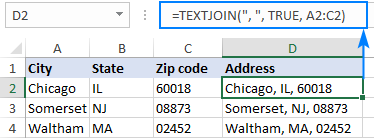
As an example, let's combine address parts from cells B2, C2 and D2 together into one cell, separating the values with a comma and a space:
With the CONCATENATE function, you'd need to specify each cell individually and put a delimiter (", ") after each reference, which might be bothersome when merging the contents of many cells:
=CONCATENATE(A2, ", ", B2, ", ", C2)
With Excel TEXTJOIN, you specify the delimiter just once in the first argument, and supply a range of cells for the third argument:
To effectively use TEXTJOIN in your worksheets, there are a few important points to take notice of:=TEXTJOIN(", ", TRUE, A2:C2)
TEXTJOIN in Excel - 6 things to remember
How to join text in Excel - formula examples
To better understand all the advantages of TEXTJOIN, let's take a look at how to use the function in real-life scenarios.
Convert column to comma separated list
When you are looking to concatenate a vertical list separating the values by a comma, semicolon or any other delimiter, TEXTJOIN is the right function to use.
For this example, we'll be concatenating wins and losses of each team from the table below. This can be done with the following formulas, which differ only in the range of cells that are joined.
For Team 1:
=TEXTJOIN(",", FALSE, B2:B6)
For Team 2:
=TEXTJOIN(",", FALSE, C2:C6)
And so on.
In all the formulas, the following arguments are used:
- Delimiter - a comma (",").
- Ignore_empty is set to FALSE to include empty cells because we need to show which games were not played.
As the result, you will get four comma-separated lists that represent wins and losses of each team in a compact form:

Join cells with different delimiters
In a situation when you need to separate the combined values with different delimiters, you can either supply several delimiters as an array constant or input each delimiter in a separate cell and use a range reference for the delimiter argument.
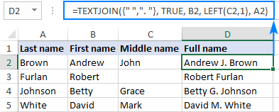
Supposing you want to join cells containing different name parts and get the result in this format: Last name, First name Middle name.
As you can see, the Last name and First name are separated by a comma and a space (", ") while the First name and Middle name by a space (" ") only. So, we include these two delimiters in an array constant {", "," "} and get the following formula:
=TEXTJOIN({", "," "}, TRUE, A2:C2)
Where A2:C2 are the name parts to be combined.
Alternatively, you can type the delimiters without quotation marks in some empty cells (say, a comma and a space in F3 and a space in G3) and use the range $F$3:$G$3 (please mind the absolute cell references) for the delimiter argument:
=TEXTJOIN($F$3:$G$3, TRUE, A2:C2)

By using this general approach, you can merge cell contents in various forms.
For example, if you want the result in the First name Middle initial Last name format, then use the LEFT function to extract the first character (the initial) from cell C2. As for the delimiters, we put a space (" ") between the First name and the Middle initial; a period and a space (". ") between the Initial and the Last name:
=TEXTJOIN({" ",". "}, TRUE, B2, LEFT(C2,1), A2)
Join text and dates in Excel
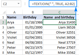
In a specific case when you are merging text and dates, supplying dates directly to a TEXTJOIN formula won't work. As you may remember, Excel stores dates as serial numbers, so your formula will return a number representing the date as shown in the screenshot below:
=TEXTJOIN(" ", TRUE, A2:B2)
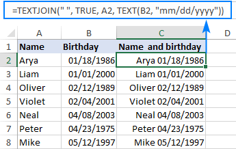
To fix this, you need to convert the date into a text string before joining it. And here the TEXT function with the desired format code ("mm/dd/yyyy" in our case) comes in handy:
=TEXTJOIN(" ", TRUE, A2, TEXT(B2, "mm/dd/yyyy"))
Merge text with line breaks
If you'd like to merge text in Excel so that each value starts in a new line, use CHAR(10) as the delimiter (where 10 is a linefeed character).
For example, to combine text from cells A2 and B2 separating the values by a line break, this is the formula to use:
=TEXTJOIN(CHAR(10), TRUE, A2:B2)
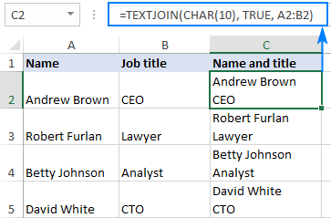
Tip. For the result to display in multiple lines like shown in the screenshot above, make sure the Wrap text feature is turned on.
TEXTJOIN IF with condition
Due to the ability of Excel TEXTJOIN to handle arrays of strings, it can also be used to conditionally merge the contents of two or more cells. To have it done, use the IF function to evaluate a range of cells and return an array of values that meet the condition to the text1 argument of TEXTJOIN.
From the table shown in the screenshot below, suppose you wish to retrieve a list of Team 1 members. To achieve this, nest the following IF statement into the text1 argument:
IF($B$2:$B$9=1, $A$2:$A$9, "")
In plain English, the above formula says: If column B equals 1, return a value from column A in the same row; otherwise return an empty string.
The complete formula for Team 1 takes this shape:
=TEXTJOIN(", ", TRUE, IF($B$2:$B$9=1, $A$2:$A$9, ""))
In a similar manner, you can get a comma-separated list of the members of Team 2:
=TEXTJOIN(", ", TRUE, IF($B$2:$B$9=2, $A$2:$A$9, ""))
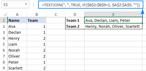
Note. Due to the Dynamic Arrays feature available in Excel 365 and 2021, this works as a regular formula, shown in the screenshot above. In Excel 2019, you must enter it as a traditional array formula by pressing the Ctrl + Shift + Enter shortcut.
TEXTJOIN IF multiple criteria
To combine the content of multiple cells with multiple conditions, you can again utilize the TEXTJOIN and IF functions together. To evaluate multiple criteria, nest them within IF's logical text using the asterisk (*) as the AND operator. This way, you'll get the logical test to return TRUE only if all the specified conditions are met.
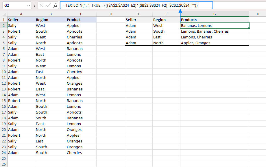
Let's break it down with an example. Suppose you want to create a comma-separated list of product names for a seller listed in cell E2 and a region in cell F2. Here's the formula you would use:
=TEXTJOIN(", ", TRUE, IF(($A$2:$A$24=E2)*($B$2:$B$24=F2), $C$2:$C$24, ""))
Here, $A$2:$A$24 contains the seller names, $B$2:$B$24 corresponds to the regions, and $C$2:$C$24 represents the product names. By locking the ranges with absolute references ($), you ensure the formula can be copied correctly to other cells.
In Excel 365 and 2021, this formula works directly as entered. In Excel 2019, remember to enter it as an array formula by pressing the Ctrl + Shift + Enter keys together.
Lookup and return multiple matches in comma separated list
As you probably know, the Excel VLOOKUP function can only return the first found match. But what if you need to get all matches for a specific ID, SKU, or something else?
To output the results in separate cells, use one of the formulas described in How to VLOOKUP multiple values in Excel.
To look up and return all matching values in a single cell as a comma-separated list, use the TEXTJOIN IF formula.
To see how it works in practice, let's retrieve a list of products purchased by a given seller from the sample table below. This can be easily done with the following formula:
=TEXTJOIN(", ", TRUE, IF($A$2:$A$12=D2, $B$2:$B$12, ""))
Where A2:A12 are seller names, B2:B12 are products, and D2 is the seller of interest.
The above formula goes to E2 and brings all the matches for the target seller in D2 (Adam). Due to the clever use of relative (for the target seller) and absolute (for the seller names and products) cell references, the formula correctly copies to the below cells and works nicely for the other two sellers too:
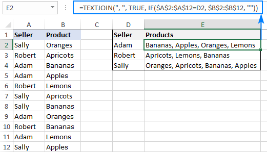
Note. As with the previous example, this works as a regular formula in Excel 365 and 2021, and as a CSE formula (Ctrl + Shift + Enter ) in Excel 2019.
The formula's logic is exactly the same as in the previous TEXTJOIN IF examples:
The IF statement compares each name in A2:A12 against the target name in D2 (Adam in our case):
IF($A$2:$A$12=D2, $B$2:$B$12, "")
If the logical test evaluates to TRUE (i.e. the name in D2 matches the name in column A), the formula returns a product from column B; otherwise an empty string ("") is returned. The result of IF is the following array:
{"";"";"Bananas";"Apples";"";"";"";"Oranges";"";"Lemons";""}
The array goes to the TEXTJOIN function as the text1 argument. And because TEXTJOIN is configured to separate the values with a comma and a space (", "), we get this string as the final result:
Bananas, Apples, Oranges, Lemons
Excel TEXTJOIN not working
When your TEXTJOIN formula results in an error, it's most likely to be one of the following:
- #NAME? error occurs when TEXTJOIN is used in an older version of Excel where this function is not supported (pre-2019) or when the function's name is misspelled.
- #VALUE! error occurs if the resulting string exceeds 32,767 characters.
- #VALUE! error may also occur if Excel does not recognize the delimiter as text, for example if you supply some non-printable character such as CHAR(0).
That's how to use the TEXTJOIN function in Excel. I thank you for reading and hope to see you on our blog next week!
 by
by
70 comments
Hi, can you help
NAME 1 SAVEMORE-CABAGAN ISABELA
NAME 1 SAVEMORE-MARKET TUMAUINI
NAME 2 SVI-BAGUIO
NAME 3 HYPER-DAGUPAN
NAME 3 SAVEMORE-CALASIAO
=TEXTJOIN(",", TRUE,IF($B$2:$B$6=NAME 1, $C2:$C6,""))
RESULT: SAVEMORE-CABAGAN ISABELA,SAVEMORE-MARKET TUMAUINI,SVI-BAGUIO,HYPER-DAGUPAN,SAVEMORE-CALASIAO
Not working , all the store was capture
Hi! If I understand the problem correctly, you should use quotes when comparing text values. Read more: IF statement for text values.
=TEXTJOIN(",", TRUE,IF($B$2:$B$6="NAME 1", $C2:$C6,""))
Hi there,
Is there a way of joining text but returning dates when there are multiple cells and the dates are placed randomly in a range, i.e., join text in cells A1:W1 where dates are in cells C1,F1,I1,M1,P1,S1,V1?
I've tried =TEXTJOIN(", ",TRUE,A1:W1(C1,F1,I1,M1,P1,S1,V1,""dd/mm/yyyy")) but that's not working...?
Sorry - typo! Formula I'm trying is: =TEXTJOIN(", ",TRUE,A1:W1(C1,F1,I1,M1,P1,S1,V1,"dd/mm/yyyy"))
Hi! Since dates in Excel are stored as numbers, you can use the ISNUMBER function to check the numbers in the cells. Use the TEXT function to write the dates in the desired format and then combine them.
Try this formula:
=TEXTJOIN(", ",TRUE,IF(ISNUMBER(C1:W1),TEXT(C1:W1,"dd/mm/yyyy"),""))
I have used the textjoin formula in plenty of files before and it worked just fine. I did the same thing on a new file and it doesnt work. I get a #value error.
The formula is =TEXTJOIN(",",TRUE,UNIQUE(G7='Auto NC'!B:B , 'Auto NC'!H:H,""))
If the value of G7 is in column B of tab Auto NC, give me the values on column H of tab Auto NC separated by commas.
This worked before in another file with extremely similar data and similar terminology. Not sure what can be causing an error on this one. The other files have way more lines to lookup and add than this one yet it works.
For example, G7=1058 . This value shows up 6 times in column B of Auto NC tab. I should be getting the 6 results from column H separated by commas, but I only get the #value error.
Column H shows the following for 1058:
NC 110450 (DispositionDraft) Rework: Draft
NC 110242 (Submitted) :
NC 109848 (DispositionDraft) Evaluation: Draft
NC 108905 (DispositionDraft) Repair: Draft
NC 107839 (WorkInProgress) Repair: InProgress
NC 107514 (DispositionDraft) Repair: Draft
I verified that the Auto NC tab doesnt have any empty cells or error cells in between values. And the 6 results add up to 246 characters which is way less than the maximum Excel can handle. Also, all the cells are in the same format, just like in the rest of my files. Not sure whats wrong. Can you please assist with this?
Thank you!
Hi! I don't think your formula can work. Try using the FILTER function. I recommend reading this guide: Excel FILTER function - dynamic filtering with formulas. For example:
=TEXTJOIN(",",TRUE,FILTER('Auto NC'!H:H,G7='Auto NC'!B:B,""))
Thank you for your quick reply, Alexander. Adding the "FILTER" gives me an empty cell, which means there's an error somewhere.
When I evaluated the formula in Excel it seems like its not reading the columns of the 'Auto NC' tab.
If I use the formula
=TEXTJOIN(",",TRUE,IF(G7='Auto NC'!$B$2:$B$20,'Auto NC'!$H$2:$H$20, ""))
and evaluate it, it shows that the formula is not reading column B of 'Auto NC'. (Instead of using the entire rows here, I just used rows 2-20 for simplicity)
The evaluation just shows as:
=TEXTJOIN(",",TRUE,IF({FALSE;FALSE;FALSE;FALSE;FALSE;FALSE;FALSE;FALSE;FALSE;FALSE;FALSE;FALSE;FALSE;FALSE;FALSE;FALSE;FALSE;FALSE;FALSE}, 'Auto NC'!$H$2:$H$20, ""))
even when the value of G7 is in that column B. All columns have the "general" format so none of them are in "text" and I have the most recent Excel version. Do you think the error has to do with having the columns of 'Auto NC' being formulas? I have used the exact formula plenty of times in more than 6 files and it reads the columns even when they are formulas. Not sure why is not working on this one.
If I evaluate
=TEXTJOIN(",",TRUE,FILTER('Auto NC'!H:H,G7='Auto NC'!B:B,""))
I get
=TEXTJOIN(",",TRUE,"")
which shows an empty cell. If I use "UNIQUE" instead of "IF" or "Filter" I get a #value error, and the result of the evaluation is the same as the "IF" evaluation I mentioned above.
Hi! The formula is working correctly. I do not know and will not guess what data you are using. If it's numbers, use the "Set prеcision as displayed" option or use rounding in formulas. If it's text, remove extra spaces and non-printable characters, as recommended here: How to remove blank spaces in Excel - leading, trailing, non-breaking.
I have a TEXTJOIN+IF formula which references several columns:
Excel Formula:
=TEXTJOIN(", ",TRUE,IF(ISNUMBER(SEARCH([@[Course or programme code]],"*"&Table18[Programme(s)/Course(s)]&"*")),Table18[Unique identifier],""))
The formula works fine when the Programmes/Courses column is the finalmost column on its table. However, I want the column to appear in the middle of the table.
I've tried copying the data over to a column in the middle several times and when I reference this column instead the formula stops working. I've tried renaming the column in case that's the issue, but it really does seem to be the placement which is the problem. Can anyone shed any light on why that might be?
Hi! It is very difficult to understand a formula that contains unique references to your workbook worksheets. Maybe this guide will be helpful: How to add or remove table rows and columns.
Hi Alexander, perhaps it will help if you just ignore the references. I've supplied some generic names in case that makes it clearer.
Essentially, I just want to know, what is the relationship between the combination of functions used below, and column placement. Evidently there is some kind of relationship but I'm struggling to find what it might be.
Excel Formula:
=TEXTJOIN(", ",TRUE,IF(ISNUMBER(SEARCH([@[Column1]],"*"&Table2[Column2]&"*")),Table2[Column3],""))
Hi! Based on your description, it is hard to completely understand your task. However, I’ll try to guess and offer you the following sample formula:
=TEXTJOIN(", ",TRUE,IF(ISNUMBER(SEARCH(Table1[@Col1],Table2[Col2])),Table2[Col3],""))
Also note that Excel spreadsheet column references are absolute and do not change when you move columns in an Excel table. Read more: Structured references in Excel tables.
Hi,
I'm trying to use TEXTJOIN to return items whose value is over 15 (number). Is there a way to ask the formula for this?
Hi! Have you tried the ways described in this blog post? If they don’t work for you, then please describe your task in detail, I’ll try to suggest a solution.
I love the textjoin function, but would like it to move through my columns from right to left instead of left to right. Is there any way I can do this?
A B C
1 paper rock scissors
I would like my textjoin to return:
"scissors, rock, paper"
Never mind - I have used helper columns to index my data and flip it 😀
Hi! To merge the values in reverse order, try this formula:
=TEXTJOIN(",",TRUE,INDEX(A1:D1,SORT(ROW(A1:A4),1,-1)))
For more information, please visit: Flip columns using formulas.
Great Article, Examples and Ideas!
but please add some More Information about "Join cells with different delimiters", and In Particular:
What happens, when the Number of Delimiters provided mismatches the Number of Text-Strings\Arguments provided?
You can easily check this yourself. If the number of delimiters is greater than the number of arguments, the delimiters will be used in order. In the example below, these are the first two delimiters.
=TEXTJOIN({","," "," ", "#","&"}, TRUE, A1:C1)
If there are more arguments than delimiters, the delimiters will be used cyclically: first, second, third, fourth, first, second, etc.
Hi - Let’s say I have the same table you have above in “ Lookup and return multiple matches in comma separated list” but Sally Smith and Sally Jones in Column A. I want to see all of the products sold by any Sally. Can I use the formula to do that? Essentially, I want to use “contains D2” to pick up all cells containing “Sally” instead of “=D2.”
Hi! To find all approximate matches, use the SEARCH function. For more information, please read: How to find substring in Excel
Try this formula:
=TEXTJOIN(", ", TRUE, IF(ISNUMBER(SEARCH(D4,$A$2:$A$12)), $B$2:$B$12, ""))
Hi!
I am using Excel 2021. I have been using TEXTJOIN for a while now. This is the formula, =TEXTJOIN(",",TRUE,IF(G:G=E11,F:F,"")), it is doing what its suppose to do, but recently I am having #NAME? error. But if I put =TEXTJOIN(",",TRUE,IF(G1:G869=E11,F1:F869,"")), it works fine. I know 869 is a weird number, but that is the maximum range that is allowing me to use the formula. Does anyone have the same problem?
Hi! Check the values in column F and G. I think there is a #NAME? error in one of the cells in these columns.
Hi, using simple textjoin for the first time in a spreadsheet that was converted from a google sheet. Every cell with textjoin =TEXTJOIN("",TRUE,BE117:CT117) that is literally it, wants to send an email when quick clicking the cell. No idea why can't change it. Thanks.
Never mind, just a dumb thing in first cell of column, deleted and fixed.
=TEXTJOIN(",",TRUE,IF(A1='Data Source'!D$2:D$51,'Data Source'!C$2:C$51,""))
I have tried this formula but not function, what's the wrong
I cannot see your problem without your data. Perhaps your Excel does not have this function. Read the instructions above carefully.
Hi sir
We have data in 2 sheets, how to match the data and text join
I'm creating a pop-up notification for my excel database to notify me of when a due date is approaching. I have all the code MOSTLY how I need it to be, but when my notification pops up, there are no commas in-between my name values, making it difficult to read the list. Can I use TEXTJOIN in my workbook code to edit my pop up? Here is what I currently have entered in the workbook:
Private Sub Workbook_Open()
Dim RenewalDateCol As Range
Dim RenewalDate As Range
Dim NotificationMsg As String
Set RenewalDateCol = Range("H3:H500") 'the range of cells that contain renewal dates
For Each RenewalDate In RenewalDateCol
'Change P2 to the cell for bring forward reminder days in the data
If RenewalDate "" And Date >= RenewalDate - Range("P2") Then
'Change the offset value to pick up the DBA Name column in the data
NotificationMsg = NotificationMsg & " " & RenewalDate.Offset(0, -7)
End If
Next RenewalDate
If NotificationMsg = "" Then
MsgBox "You do not need to renew any DBAs today."
Else: MsgBox "The following DBAs need renewal: " & NotificationMsg
End If
End Sub
Sorry, we don't provide VBA coding help.
Is it possible to use TEXTJOIN with multiple delimiters, where one of those delimiters is a line break?
I tried this but it didn't work =TEXTJOIN({"-","Char(10)"},TRUE,C12:C15)
Thanks
Hi!
Please try the following formula:
=TEXTJOIN("-"&CHAR(10),TRUE,C12:C15)
Don't forget to set the cell format to Wrap text.
Can you have a dynamic delimiter?
I want to join text like a sentence from a list of items. I want the items to be combined using "," but the last item should be combined with ", &". However long my list is the last item should be combined with the later.
Hello!
Use the TEXTBEFORE and TEXTAFTER functions to insert the desired character after the last comma.
=TEXTBEFORE(A1,",",-1)&",&"&TEXTAFTER(A1,",",-1)
I hope it’ll be helpful.
Hello!
Do you know if it's possible to combine the line break delimiter with finding multiple matches?
I tried this, but it doesn't function properly, with or without the CSE:
=TEXTJOIN(CHAR(10), TRUE, IF($A$2:$A$12=D2, $B$2:$B$12, ""))
Thanks!
Hello!
I don't really understand what you want to do. But maybe you will find this article useful: How to VLOOKUP multiple values in Excel with criteria. If this does not help, explain the problem in detail.
Hello!
Can you use TEXTJOIN in multiple sheets?, example: TEXTJOIN(", ",TRUE,IF($C9='5-Sale'!$D$10:$D$10009,'5-Sale'!$H$10:$H$10009,""))). I use this formula and it displayed #VALUE. can you fix this or any advice?
Hope to hear from you soon. Thank you!!
Hello!
Perhaps the error occurs because the TEXJOIN function can join no more than 252 text arguments.
Please help with suitable formula:
Input in 3 columns:
A B C
Morning Adam Good
Afternoon Bob
Evening James
Alice
Sam
Pete
Desired Result in Column continuous sentences:
Good Morning Adam
Good Morning Bob
Good Morning James
Good Morning Alice
Good Morning Sam
Good Morning Pete
Good Afternoon Adam
Good Afternoon Bob
Good Afternoon James
Good Afternoon Alice
Good Afternoon Sam
Good Afternoon Pete
Good Evening Adam
Good Evening Bob
Good Evening James
Good Evening Alice
Good Evening Sam
Good Evening Pete
Using excel how to get the output from the below input
Input
Name Task
a 1,2,3,4
b 5,6,7,8
c 9,10,11,12
d 13,14,15,16
Output:
Name Test
a 1
a 2
a 3
a 4
b 5
b 6
b 7
b 8
c 9
c 10
c 11
c 12
d 13
d 14
d 15
d 16
How to retain formatting of specific cell or cells while textjoin - for example: out of three cells being joined, only one was bold. In the textjoin cell, I want that value to retain its bold formating
Hi!
Excel formulas cannot change cell formatting. This can be done using a VBA macro.
Hello,
i've been trying using formula's to merge the bundle_Id values in one cell which have similar number to the different sheet but I am not able to merge them. Using =TEXTJOIN(",",true,B2:B9) and which is working well but have to merge the cells individually. Can you please suggest some formula on this.
Example -
bundle_id sku formula
1 75613 1
1 75176 1
1 74207 1
1 74301 1
1 62750 1
1 74378 1
1 74299 1
1 37738 1
2 75613 1
2 75176 1
2 74205 1
2 74301 1
2 62750 1
2 74378 1
2 74299 1
2 37738 1
Just like this i want to merge all 2 values in one column for 4000 row together. How can i merge them
Hi!
I am not sure I fully understand what you mean. If I understand correctly, your example has 3 values per line. Explain what you want to merge. Write an example of the result.
Hi,
I have an SAP extract for Special Instructions.
In SAP, for the same Special Instruction, I may have 1 or more lines of text and those lines need to be grouped into a single cell for each unique Customer ID.
What I need to do is combine the cells with a formula (which is the easy part) but I want to the formula to detect when the ID in column A changes to another accountID.
So 6 lines of data in Cell C1to C6 are combined and the formula detects that the ID changes to a new ID (from 10000 to 10001) and combines cells C7 to C9, and then C10 to C15...
Cust# Text ID Remit To Text
10000 0009 Remit to:
10000 0009 PERKINELMER Optoelectronics
10000 0009 c/o ROYAL BANK OF CANADA
10000 0009 1, Place Ville Marie
10000 0009 Montréal (QC) H3C 3A7, Canada
10000 0009 Account #403
10001 0009 Remit to: EG&G Optoelectronics
10001 0009 P.O. Box 66512 AMS O'Hare
10001 0009 Chicago, IL 60666-0512 USA
10002 0009 Remit to: EG&G Optoelectronics
10002 0009 P.O. Box 66512 AMS O'Hare
10002 0009 Chicago, IL 60666-0512 USA
10003 0009 Remit to:
10003 0009 EG&G CANADA Ltd. Optoelectronics
10003 0009 c/o ROYAL BANK OF CANADA
10003 0009 1, Place Ville Marie
10003 0009 Montréal (QC) H3C 3A7, Canada
10003 0009 Account #124
Hope this makes sense! :)
Hi,
Is there anyway to combine two delimited lists term by term.
For example cell A1 has 1,2,3,4 and cell B1 has 5,6,7,8. I would like cell C1 to have 1,5 ; 2,6 ; 3,7; 4,8.
The textjoin function seems to only concatenate cells end to end without being able to enter the cells and go term by term. Any help would be appreciated.
Thanks.
Hello!
I think it is impossible to solve your problem with the help of one formula. You need to split the text into cells, and then combine their values in the desired order.
Hi, is there a way to combine text from multiple columns into one cell, but only returning unique values? I've been using the formula =textjoin(", ", true, G4:R4) which works well but some of the cells have duplicated values. EG:
O P Q R S
1.Apple Pear Orange Apple Apple, Pear, Orange, Apple
2. Pear Pear Pear Pear Pear, Pear, Pear, Pear
What I'm getting in column 'S' (where the formula is): row1:Apple, Pear, Orange, Apple. row2: Pear, Pear, Pear, Pear but I only want it to show one of each value, so row1: pear, orange; row 2: Pear. I tried to prefix the formula with =unique but that still returns the duplicate word or phrase.
Any suggestions would be most welcome!
Hello!
You can extract unique values from the band using the formula in this comment.
I hope I answered your question. If something is still unclear, please feel free to ask.
Thankiu so much
Hello I am trying to use this to get a date/ time results however it's giving this result :
44378.57784,44378.48631,44378.44199
=ARRAY_CONSTRAIN(ARRAYFORMULA(TEXTJOIN(",",TRUE,IF(Sheet1!A2=C:C,A:A,""))), 1, 1)
Thank You for posting this tutorial.
Is there a way to use a macro to use Textjoin to put multiple types of items in the same cell, with each items having a different color based on a value of type of item?
So, I have this table, and I want a single cell, where each of the items for the same date are together, but are a different font color depending on the calendar type. So, line 2 and line 5 would be the same color.
DATE Calendar Time Description UNIQUE VALUE (CALCULATED)
12/23/2021 Personal 6AM-Fitness Training 44553|1
12/23/2021 Kids 7AM-Schools closed 44553|2
12/23/2021 Family 3PM-Holiday Break begins 44553|3
12/23/2021 Peter 5PM-Jiu Jitsu 44553|4
12/24/2021 Kids 7AM-Schools closed 44554|1
Hi!
You can paint a part of a cell with a special color only manually. Excel formulas don't work here.
Hi, the cells returned "N/A" in lookup and return multiple matches in comma separated list, but when i remove some rows in the lookup table, it works. Is there a limit on how many rows in a lookup table this function can handle, how many rows?
Hi,
Can we edit range as per condition in textjoin.
Example i have pivot table, in which i have the numbers of the range to textjoin,
But i have to edit those range as per the pivot value, is there any formula in which the range get automatically selected as per the pivot table value .
Hello!
The INDIRECT function is used to convert a value to a cell address. Perhaps this article will be useful to you.
Hi! How can I use textjoint to give me the 5 highest values across multiple columns in excel 365? The values should reference to the respective left adjacent cells and each of the five top values should return more than one matching value, if any. I hope I make myself understood
Hello!
To find the 5 highest values in columns, I recommend using the LARGE function as described in this article. The value from the cell will be returned, but not the reference from that cell. You can combine these values using the TEXTJOIN function as described in the article above.
I have been able to successfully combine my text using the instructions provided, but now I need to copy the combined text into another spreadsheet. How do I do this since the content of the cell is a formula?
Hi,
Here is the article that may be helpful to you: How to copy values in Excel
I hope it’ll be helpful.
#VALUE! error occurs if the resulting string exceeds 32,767 characters.
Please help to resolve the error.
Hi
I want to use "Join cells with conditions" this formula When ever i use " =TEXTJOIN(", ", TRUE, IF($B$2:$B$9=1, $A$2:$A$9, "")) " this formula it show "#VALUE!" & i also used "Return multiple matches" =TEXTJOIN(", ", TRUE, IF($A$2:$A$12=D4, $B$2:$B$12, "")) " this one too but it's some times Blank in cell. Please help me in this case
Hello!
Unfortunately I was unable to reproduce your error. Therefore, the question is not clear to me.
Please provide me with an example of the source data and the expected result.
When i used TEXTJOIN formula then i saw some of the cell values are incorrect & Some of the cells are blank too. i want to share my excel file for the error but there is no option for attachment.
Hello Svetlana,
Do you have a suggestion for an alternative or workaround for the 256 char. limit of the if function when used within a textjoin function? I am wanting to join text in column AD if it's corresponding code in column Q is 8. For example, =TEXTJOIN("; ";TRUE;IF($Q$2:$Q$22=8;$AD$2:$AD$22;"")). It works perfectly unless the text in any of the cells is greater than 256 (if function limitation), the formula returns #VALUE!.
Hi,
I tried using the formula above, but it is giving me all the values in column B separated by a comma
Hello!
Please describe your task in more detail - what you are trying to find, what formula you used, and what problem or error occurred. Give an example of the source data and the expected result.
It’ll help me understand it better and find a solution for you. Thank you.