On the web, there are many questions about how to create an expandable drop-down list that can be copied across multiple rows and very few answers. Here's a working solution.
The introduction of dynamic arrays has made our lives as Excel users a lot easier. Among many other things, they significantly simplify the creation of dynamic drop down lists. The above-linked tutorial shows how to quickly set up a multiple drop-down with dynamic arrays and make it expandable to automatically include new entries.
I felt very proud of the work we'd done until we got a few comments like this: "That works great for one row, but how to get this to work for the entire column?" A fair question. Indeed, Excel picklists are most often used in worksheets with hundreds of rows to facilitate data entry. So, we reconsidered the whole approach, worked out a formula that automatically adjusts for each row, and I'm thrilled to share this new solution with you!
Important note! Because this solution relies on the dynamic array feature, it is only applicable in Excel for Microsoft 365 and Excel 2021. In pre-dynamic versions of Excel, please use the traditional approach to creating multiple dependent drop down lists.
Source data
For starters, let's get some source data to work on. In our main table on the left, we want to have two picklists in each row, so that selecting a Dept. in the first list only displays Managers for that selected department in the second list. If you change the selection in the main list, the names in the dependent drop-down will update accordingly.
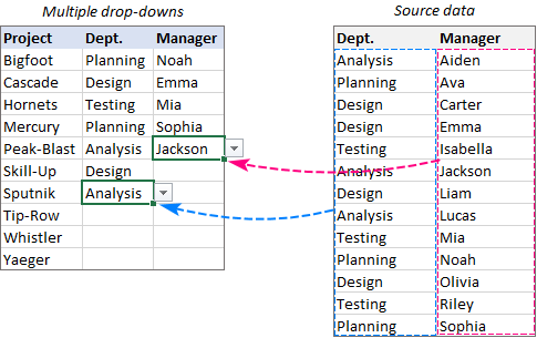
Step 1. Structure source data
The source data for drop-down lists often come from different sources and are organized differently. So, our first step is to structure the original data according to our needs. For this, we are going to create some sort of preparation table that will list all different department names in the header row, and under each dept. name there will be a list of employees working in that specific department. To automate the work and prevent human errors, we will be using the following formulas.
To get the departments, enter this formula in H2.
=TRANSPOSE(SORT(UNIQUE(E3:E15)))
Here, the UNIQUE function extracts all the different departments from E3:E15. The SORT function arranges the results in alphabetical order so that the items of your main list will be sorted from A to Z (if you don't want that, you can remove SORT from the formula, and the dept. names will appear in the same order as in your source table). Finally, TRANSPOSE changes the output orientation from vertical to horizontal.
Please notice that the formula needs to be entered just in one cell, and the results spill into neighboring cells automatically (this feature is called a spill range).
This way, we've got the items for our main drop-down list:
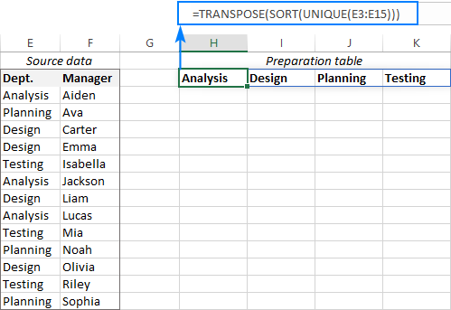
To pull the manager names, the formula in H3 is:
=SORT(FILTER($F$3:$F$15, $E$3:$E$15=H$2))
Here, we utilize the FILTER function to filter the employees that belong to a particular department ($E$3:$E$15=H$2). The SORT function arranges the names in alphabetical order (if you wish to preserve the existing order, remove it from the formula).
Like the previous formula, this one is also dynamic, and the whole spill rage is filled with the results at once. All you need to do is to drag the formula to the right to get a list of managers for each dept.
And this gives us the items for the dependent drop-down list:
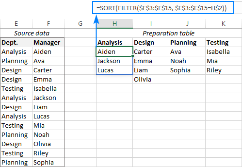
Tips and notes:
- In this example, we have all the data on the same sheet to make things easier for you to follow. In your real spreadsheets, you'd better place a preparation table on a separate sheet to make sure there are enough empty cells down and to the right to accommodate all the data. As already mentioned, dynamic arrays formulas are entered only in one cell, and you cannot know how many cells the results will spill into.
- If your goal is to make expandable drop-down lists, then use a slightly different method for the preparation table, which is discussed in this example.
Step 2. Make a primary drop-down list
With the source data properly arranged, create the first drop-down list in the usual way with the help of Excel Data Validation:
- Select the topmost cell in which you want the primary dropdown list to appear (B3 in our case).
- On the Data tab, in the Data Tools group, click Data Validation.
- On the Settings tab of the Data Validation dialog box, configure the rule:
- Under Allow, select List.
- In the Source box, enter the spill range reference pointing to the departments names in the preparation table: =$H$2#
This syntax (cell address followed by a hash tag) refers to the entire spill range no matter how many cells it actually contains.
- Click OK to close the dialog.
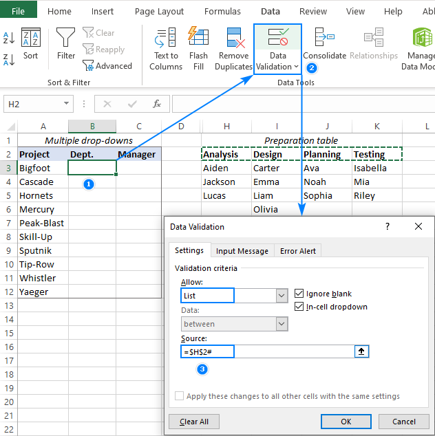
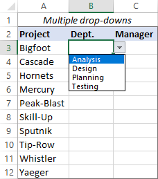
The primary drop-down list for the first cell is done:
Step 3. Create a dependent drop-down list
Technically, setting up a successive picklist seems pretty easy - you just need to create one more data validation rule for another column. However, there's a tricky part - the formula for the Source box. This time, you cannot use a normal spill range reference because the second drop-down list needs to take into account the selection in the first drop-down. To solve this need, we'll be referring to a relevant spill range indirectly with this formula:
Where:
- row_num - the number of the row in the preparation table in which the formula returning the items for the dependent dropdown resides. Our formula is in row 3 (H3:K3), so it's 3. Instead of hardcoding the row number, you can use the ROW() function, but we won't complicate things more than they already are.
- preceding_col - a cell reference to the column preceding the leftmost column of the preparation table. In this example, the preparation table begins in H2. The preceding column is G, so we use COLUMN(G1). Here, only the column coordinate matters, the row number can be any.
- dropdown_cell - is the address of the topmost cell containing the primary drop down list, B3 in our case. Please be sure to use a relative cell reference without the $ sign, so that the formula adjusts correctly for each row where you'll copy your drop-down.
- dropdown_spill_range - the reference to the spill range in the preparation table containing the items for the primary drop down list. In our example, it's the departments returned by the dynamic array formula in H2, so we use this spill range reference: $H$2#
Putting all the above pieces together, we get the following formula for the dependent drop down validation rule:
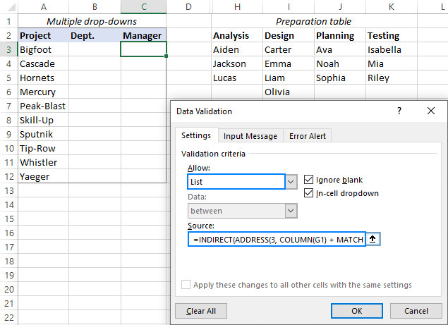
=INDIRECT(ADDRESS(3, COLUMN(G1) + MATCH(B3, $H$2#, 0), 4) & "#")
Now, simply select the topmost cell for the secondary drop-down list (C3), go to the Data tab > Data Validation, and configure the rule like this:
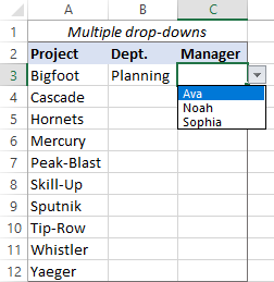
That's it! The dependent drop-down list is good to go:
Tip. If your source data and the preparation table are on another sheet, then include the sheet name in the lookup_array argument of MATCH, and also concatenate it with the cell reference within INDIRECT like this:
=INDIRECT("Sheet1!"&ADDRESS(3, COLUMN(G1) + MATCH(B3, Sheet1!$H$2#, 0), 4) & "#")
In the above formula, simply replace Sheet1! with the name of the worksheet where your source data and the preparation table are kept.
How this formula works:
From my experience, many of our blog visitors are eager to know not only how to apply this or that formula but also understand its internal logic. For such curious and thoughtful users, I'm providing the detailed break-down of the formula:
=INDIRECT(ADDRESS(3, COLUMN(G1) + MATCH(B3, $H$2#, 0), 4) & "#")
On a high level, we utilize the INDIRECT function to "dynamically" refer to the spill range of managers corresponding to the department selected in the primary dropdown.
Suppose you picked Planning from the drop-down in B3. The employees of the Planning dept. are listed in column J beginning in J3. That means, we need to somehow supply the J3# reference to INDIRECT, and here's how we do it:
To get the column letter, the following 3 functions are used together:
ADDRESS(3, COLUMN(G1) + MATCH(B3, $H$2#, 0), 4)
The COLUMN function returns the column number of G1, which is 7.
The MATCH function searches for the B3 value in list of departments beginning in H2 and return its relative position, which is 3 (Analysis, Design, Planning, …).
Adding up these two numbers gives us 10, so the ADDRESS function takes this form:
ADDRESS(3, 10, 4)
Where 3 is the row number, 10 is the column number and 4 is the relative cell reference type. The result is the "J3" reference that goes directly to INDIRECT :) and reduces our tricky formula to an easy understandable one:
INDIRECT("J3"&"#")
Concatenating a cell reference with a hash tag produces a spill range reference, so that INDIRECT returns an entire array rather than a single cell value. Done!
The beauty of this formula is that it works perfectly for a single-letter, two-letter and even tree-letter column (thank you Jonathan for pointing us in the right direction!).
Step 4. Copy drop down lists across multiple rows
This is the easiest part. For the picklists to appear in multiple cells, you can simply copy them like any other cell content by using the Copy / Paste feature or by dragging through the adjacent cells. For practice, we will try both techniques.
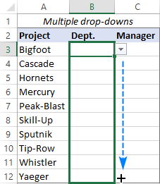
To copy the primary drop down list, select the cell containing it (B3) and drag the fill handle (a small square at the lower right-hand corner of the cell) through as many cells as needed:
To copy the dependent drop down list, let's do a regular copy/pasting:
- Select the cell with the secondary drop-down (C3) and press Ctrl + C to copy it.
- Select all other cells where you want the dependent list to appear (C4:C12) and press Ctrl + V to paste the copied contents.
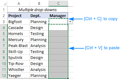
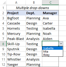
Now, both picklists appear in every row letting you select a department and manager for each project.
Please keep in mind that the above methods copy all the contents of a cell including Data Validation and the current selection. So, they are best to be used when no item has been selected in the list yet.
If you've already selected the items, then you can use the Paste Special feature to copy the Data Validation rule.
Result: multiple rows dependent drop down list
Though our dynamic arrays solution is not a one-click setup, it's a way faster than it looks and definitely much faster than the old-fashioned approach with named ranges. Anyway, the result is worth the effort, agree?
Here it is - a multi-level drop down for multiple rows where selecting an item from the first list determines which items will appear in a secondary drop-down.
How to make multiple drop-down list expandable
If more data is likely to be added to your source table in the future and you wish to have new entries included in the drop-down lists automatically, then you will have to use a bit more complex versions of the formulas for the preparation table. There are 2 possible approaches here, a regular range and a full-fledged Excel table, each having its own caveats.
Approach 1. Organize source data in a table
One of the key advantages of Excel tables is automatic expansion to accommodate new data, and we are going to leverage this ability.
The first thing you do is convert source data to a table. The quickest way is to select the range E2:F15 and press Ctrl + T. For convenience, we name the table Source_data.
Next, build the formulas for the preparation table by using structured references. If you are not familiar with this syntax, it's not a problem! Just start typing a formula in a cell, select the required range in your table, and Excel will create an appropriate structured reference for you automatically based on the column names.
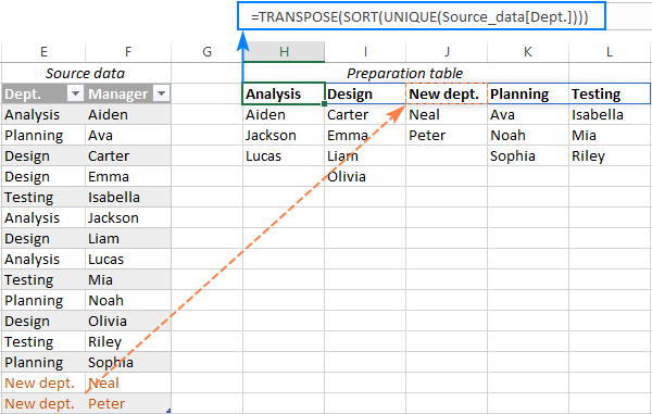
To extract the departments, the formula in H2 is:
=TRANSPOSE(SORT(UNIQUE(Source_data[Dept.])))
To get the manager names, enter the below formula in H3 and drag it to the right through a few more cells than there currently departments (say, through P3):
=IFERROR(SORT(FILTER(Source_data[[Manager]:[Manager]], (Source_data[[Dept.]:[Dept.]]=H$2))),"")
Play pay attention that absolute structured references should be used for the Dept. and Manager columns so the references won't shift when the formula is copied horizontally. The default in Excel tables is a relative column reference such as table[column]. To make the reference absolute, you need to repeat the column name like this: table[[column]:[column]].
The IFERROR function is used to prevent errors when the formula is copied to extra columns to the right.
If all done correctly, the preparation table expands automatically to incorporate new records:
Approach 2. Use a range but improve formulas
If the table references look too complex to you, you can do with a normal range too. In this case, a couple of improvements need to be made to the formulas:
- Include some empty rows in the ranges supplied to both formulas.
- Filter out blank cells so they won't get into your picklists.
To extract the department names, the formula in H2 is:
=TRANSPOSE(SORT(UNIQUE(FILTER(E3:E30, E3:E30<>""))))
Please pay attention that we use the range E3:E30, though currently there are far fewer records in our source table.
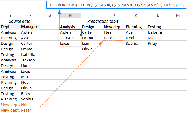
To get the manager names, enter the below formula in H3 and drag it through a few more columns than there are currently entries in the header row:
=IFERROR(SORT(FILTER($F$3:$F$30, ($E$3:$E$30=H$2)*($E$3:$E$30<>""))),"")
In this case, we lock the range references with the $ sign to prevent them from changing while copying the formula.
As with the previous solution, the new records appear in the preparation table once they are added to the source table.
Result: expandable multiple drop-down list
Whichever approach you opted for, configure and copy two Data Validation rules like explained in Steps 2 - 4 above, and the newly added items will be displayed in the drop-down lists without any extra effort on your side!
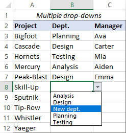
That is my go-to for making a multi-level dropdown for every row in Excel. Hopefully, this solution will be useful for you too. Anyway, I thank you for reading and hope to see you on our blog next week!
Practice workbook for download
Multiple rows dependent drop-down (.xlsx file)
 by
by
134 comments
I keep getting REF error messages when I adjust the formula to pull from another tab
=INDIRECT('LookupTables2'!&ADDRESS(3,COLUMN(C1) + MATCH(D2,LookupTables2!$D$2#,0),4) & "#")
I have attempted to use double quotes, single quotes and every combination for the formula before the address part but this still errors out. when I don't add any tab name before the address part and I have the formula on the same tab as lookupTables2 the formula works
what am I missing?
Hi! I can't check your formula because I don't have your data. However, the function MATCH(D2,LookupTables2!$D$2#,0) returns the error #REF!
The # symbol is only used in structured references.
It's not necessary for standard cell references.
When you specify a worksheet name in a reference, it is not a structured reference, but an external reference.
Maybe this article will be helpful: Structured reference in Excel tables
Hi! Can you please create a workbook where the source data are in a new sheet? I can't work out the formula for the dependent list with source data in a different sheet.
Hi! I cannot create a workbook for you on your computer. However, if you download the sample file that is linked at the end of this article, you will be able to see how to create a drop-down list of source data on a different worksheet. Detailed instructions are also available here: Change dropdown based on named range.
I see no place to post my test results. I am asking for assistance on fixing my error. The download example does show an example of the look up results on another tab. It only shows everything on the same tab.
Hi! Try to follow the recommendations from this article: How to evaluate and debug formulas in Excel.
Hello, I have followed along with this tutorial and have gotten the first dependent column to work as described. I'm a test scheduler for a University. Currently, we manually type in the course, number, and instructor name. What I'd like to do, is pick from drop down for Course (A), have the second column only show the course numbers that apply to the chosen course (B), then have the third column only show the instructors for that specified course number (C), and then of course this needs to be copied down the sheet (appointment times). That part I'm okay on.
Right now, A & B work. I can't get C to work. When I modified the '=INDIRECT' code in the data validation box for the third column, it only shows me the instructors for the first course in the list.
My data set is huge, obviously. I have it set up in a table and it's 987 rows deep. I followed the steps to do the spill formula horizontally for my Course Names, then did the same thing for the Course Numbers. The Course Names only took up one row, but since there are more possibilities for course numbers, these took up multiple rows. I followed the same steps to do the spill range for Instructors, but ended up having to put that some 35 rows underneath the other 2 spill ranges.
I went back and read the instructions for multiple dependent drop downs (https://www.ablebits.com/office-addins-blog/create-dynamic-dependent-drop-down-excel/) but I don't think that will work for my specific use case.
Can you assist on getting the third dependent drop down working?
Hello! As you understand, I can't create a drop-down list for you in your workbook. Try to follow the recommendations from this article: Making a dependent (cascading) drop down list in Excel.
Hi, thank you so much, that is very helpful !
Quick follow-up using the same example. What if we need multiple levels for the dropdown. In this case more than 2 columns. Like the "Project" column would also depend on a list of let's say "clients" ? Would that be doable with a dynamic approach ?
Best
MB
Hello! You can add as many levels of dependent dropdown lists as you need. If you want a dropdown list to depend on two previous dropdown lists, see the recommendations in the previous comment below.
I hope it’ll be helpful. If this is not what you wanted, please describe the problem in more detail.
Hi Alexander,
Thanks for this post, it's great!
Is it possible to add additional level of dependencies in subsequent columns??
I'm working on a spreadsheet that has the following:
Column A = Region (e.g. Auckland, Queenstown etc)
Column B = Service Type (e.g accommodation, transfer etc)
Column C = Supplier Name (e.g Hotel ABC)
Column D = Service Description (e.g. Hotel Room, Suite, Penthouse etc)
Based on the information above, I have the Column A & B lists in place (i.e. the list in Column B reflects the choice in Column A. Thanks again for that!!
Can I amend the formula so that the list in Column C reflects the choices of BOTH Columns A and B? (and then so that the list in Column D reflects A,B, and C).
Regards
V.
Hello! You can create a third drop-down list that depends on the first and second drop-down lists. We have a special tutorial that can help to solve your problem: How to make a dynamic dependent dropdown list in Excel an easy way.
I hope it’ll be helpful.
Hi,
Does the solution for having a 3rd (or even 4th, 5th, etc.) drop-down list that is dependant on the 1st & 2nd lists apply to this article, i.e. can this solution work for multiple rows that need to have the same drop down lists?
Hi! Of course, this solution can be used for the third and more levels of dependent drop-down lists. You can see other ways to create dependent drop-down lists by clicking here: Making a dependent (cascading) drop down list in Excel.
Thanks for the response but I'm not sure the article you have shared is relevant. I am trying to set up a dependent drop-down list for multiple rows in Excel using the solution described in this article. However, I would like to use this solution for more than 2 dependent drop-down lists. I cannot see how that is possible. In your example above, I would require a 3rd dropdown dependent on the Manager selected in the 2nd dropdown. Can you advise how this would work, what the preparation table would look like and what the steps would be?
Create another array "Source data1" (for example, in columns M and N), where in column M - Manager, in column N - data for the third drop-down list depending on the selected Manager. Repeat all the steps described in the article above.
I am having an issue with getting the error of "The Source currently evaluates to an error. Do you want to continue?"
Using the formula: =INDIRECT("Structure_InsurancePlanList!" & ADDRESS(ROW(),COLUMN(A1) + MATCH(Claims!C4,Structure_InsurancePlanList!$B$1#,0),4)&"#")
My Source Data is in worksheet InsurancePlanList's table InsurancePolicyPlanList (Column A: PlanName; Column B: PolicyNumber; Column C:Type)
My Structured Source Data is in the worksheet Structure_InsurancePlanList, starting in Column B (Column A is blank)
B1 =TRANSPOSE(SORT(UNIQUE(IF(UNIQUE(PlanTypes!$A$3:$A$18,FALSE,FALSE)=0,"",UNIQUE(PlanTypes!$A$3:$A$18,FALSE,FALSE)),FALSE,FALSE),,1,FALSE))
B2 (and the rest of row 2) =SORT(IFERROR(UNIQUE(IF(FILTER(InsurancePolicyPlanList[[PlanName]:[PlanName]],InsurancePolicyPlanList[[Type]:[Type]]=Structure_InsurancePlanList!B$1)=0,"",FILTER(InsurancePolicyPlanList[[PlanName]:[PlanName]],InsurancePolicyPlanList[[Type]:[Type]]=Structure_InsurancePlanList!B$1)),FALSE,FALSE),""))
Any thoughts on how I can fix this?
Hi! I can't check a formula that contains unique references to your data, which I don't have.
DOES THIS METHOD WORK ON EXCEL WEB VERSION?
We have said many times that VBA does not work in Excel for Web.
Is this VBA though? I can't see why it wouldn't work on Excel for web, and yet it doesn't appear to... Any suggestions would be gratefully received!
Thank you for a fantastic tutorial in any case :D
Hi! This question has already been asked in the comments. Microsoft Office for the web does not support VBA.
Well aware of that, but as I say this tutorial doesn't seem to use any VBA functionality?? Unless I am missing something...
Hi! If you are not using VBA, all functions will work. You can download the sample file from the link at the end of the article and open it in Excel Online.
My source data is already all organized manually the same way as your "preparation table" without formulas, so I was essentially starting at step #2 but I keep getting an error "The Source currently evaluates an error". How to fix?
My formula is:
=INDIRECT("Sheet1!"&ADDRESS(4, COLUMN(L1) + MATCH(B5, Sheet1!$M$3:$T$3, 0), 4) & "#")
Hi! Unfortunately, I can't see your data and can't create a dropdown list for you in your workbook.
I am getting the following error message: Inconsistent Calculated Column Formula. What could it be?
Hi! I can't see your data and your formulas. So I can't help you without having the necessary information.
Great tutorial!!
Question - if a change is made in Dept is there a way to change Manager to blank (prompting a reselection of Manager) to prevent mismatched information in the table?
Hi! You can automatically delete a value in a cell with a second-level drop-down list when you change the first-level drop-down list using VBA. This cannot be done using formulas.
Thanks a lot. This was very informative and perfectly explained method.