The tutorial gives a brief introduction to the ADDRESS function syntax and shows how to use it to return an Excel cell address and more.
To create a cell reference in Excel, you can type the column and row coordinates manually. Alternatively, you can get an Excel cell address from the row and column numbers supplied to the ADDRESS function. Almost pointless on its own, in combination with other functions this technique can be the only solution in situations when it is not possible to refer to a cell directly.
Excel ADDRESS function - syntax and basic uses
The ADDRESS function is designed to get a cell address in Excel based on the specified row and column numbers. A cell address is returned as a text string, not an actual reference.
The function is available in all versions of Excel for Microsoft 365 - Excel 2007.
The syntax of the ADDRESS function is as follows:
The first two arguments are required:
row_num - the row number to use in the cell reference.
column_num - the column number to build the cell reference.
The last three arguments, which specify the cell reference format, are optional:
abs_num - the reference type, absolute or relative. It can take any of the below numbers; the default is absolute.
- 1 or omitted - absolute cell reference like $A$1
- 2 - mixed reference: relative column and absolute row like A$1
- 3 - mixed reference: absolute column and relative row like $A1
- 4 - relative cell reference such as A1
a1 - the reference style, A1 or R1C1. If omitted, the default A1 style is used.
- 1 or TRUE or omitted - returns the cell address in the A1 reference style where columns are letters and rows are numbers.
- 0 or FALSE - returns the cell address in the R1C1 reference style where rows and columns are represented by numbers.
sheet_text - the name of the worksheet to include in the external reference. The sheet name should be supplied as a text string and enclosed in quotation marks, e.g. "Sheet2". If omitted, no worksheet name is used, and the address defaults to the current sheet.
For example:
=ADDRESS(1,1) - returns the address of the first cell (i.e. the cell at the intersection of the first row and first column) as an absolute cell reference $A$1.
=ADDRESS(1,1,4) - returns the address of the first cell as a relative cell reference A1.

In the following table, you will find a few more reference types that can be returned by ADDRESS formulas.
| Formula | Result | Description |
| =ADDRESS(1,2) | $B$1 | Absolute cell reference |
| =ADDRESS(1,2,4) | B1 | Relative cell reference |
| =ADDRESS(1,2,2) | B$1 | Relative column and absolute row |
| =ADDRESS(1,2,3) | $B1 | Absolute column and relative row |
| =ADDRESS(1,2,1,FALSE) | R1C2 | Absolute reference in the R1C1 style |
| =ADDRESS(1,2,4,FALSE) | R[1]C[2] | Relative reference in the R1C1 style |
| =ADDRESS(1,2,1,,"Sheet2") | Sheet2!$B$1 | Absolute reference to another sheet |
| =ADDRESS(1,2,4,,"Sheet2") | Sheet2!B1 | Relative reference to another sheet |
How to use ADDRESS function in Excel - formula examples
The below examples show how to use the ADDRESS function inside bigger formulas to accomplish more difficult tasks.
Return a cell value in a given row and column
If your goal is to get a value from a specific cell based on its row and column numbers, use the ADDRESS function together with INDIRECT:
The ADDRESS function outputs the cell address as text. The INDIRECT function turns that text into a normal reference and returns the value from the corresponding cell.
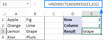
For example, to get a cell value based on the row number in E1 and the column number in E2, use this formula:
=INDIRECT(ADDRESS(E1,E2))
Get the address of a cell with the highest or lowest value
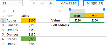
In this example, we'll first find the highest and lowest values in the range B2:B7 by using the MAX and MIN functions and output those values into special cells:
Cell E2: =MAX(B2:B7)
Cell F2: =MIN(B2:B7)
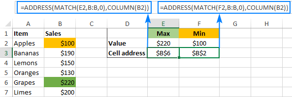
And then, we'll use ADDRESS in combination with the MATCH function to get the cell addresses.
Cell with the max value:
=ADDRESS(MATCH(E2,B:B,0), COLUMN(B2))
Cell with the min value:
=ADDRESS(MATCH(F2,B:B,0), COLUMN(B2))
In case you do not want the highest and lowest values in separate cells, you can nest the MAX/MIN function in the first argument of MATCH. For example:
Cell with the highest value:
=ADDRESS(MATCH(MAX(B2:B7),B:B,0), COLUMN(B2))
Cell with the lowest value:
=ADDRESS(MATCH(MIN(B2:B7),B:B,0), COLUMN(B2))
How these formulas work
To find the row number, you use the MATCH(lookup_value, lookup_array, [match_type]) function that returns a relative position of lookup_value in lookup_array. In our formula, the lookup value is the number returned by the MAX or MIN function, and the lookup array is the entire column. Consequently, a relative position of the lookup value in the array exactly matches the row number on the sheet.
To find the column number, you use the COLUM function. Of course, nothing prevents you from typing the number directly in the formula, but COLUMN saves the trouble of manual counting in case the target column is in the middle of the sheet.
Get a column letter from a column number
To turn any given number into a column letter, use the ADDRESS function inside of SUBSTITUTE:
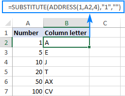
As an example, let's find the column letter corresponding to the number in A2:
=SUBSTITUTE(ADDRESS(1,A2,4),"1","")
Looking at the results below, we can say that the first column on the sheet is A, which is obvious; the 10th column is J, the 50th column is AX, and the 100th column is CV:
How this formula works
For starters, set up the ADDRESS function to return a relative reference to the first cell in the target column:
- For the row number, use 1.
- For the column number, supply the reference to the cell containing the number, A2 in our example.
- For the abs_num argument, enter 4.
As the result, ADDRESS(1,A2,4) would return A1.
To get rid of the row coordinate, wrap the above formula in the SUBSTITUTE function and replace "1" with an empty string (""). Done!
Get the address of a named range
To find the address of a named range in Excel, you will first need to obtain the first and last cell references, and then join them together. This works a bit differently in pre-dynamic Excel (2019 and older) and Dynamic Array Excel (Office 365 and Excel 2021). The below examples are for Excel 2019 - Excel 2007. The instructions for Excel 365 and Excel 2021 are here.
How to get address of the first cell in a range
To return a reference to the first cell in a named range, use this generic formula:
Assuming the range is named "Sales", the real formula goes as follows:
=ADDRESS(ROW(Sales), COLUMN(Sales))
And returns the address of the upper left cell in the range:
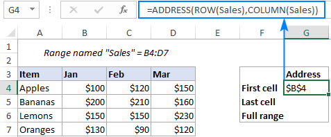
In this formula, the ROW and COLUMN functions return an array of all the row and column numbers in the range, respectively. Based on those numbers, the ADDRESS function builds an array of cell addresses. But because the formula is entered in a single cell, only the first item of the array is displayed, which corresponds to the first cell in the range.
How to get address of the last cell in a range
To find the address of the last cell in a named range, use this generic formula:
Applied to our range named "Sales", the formula takes the following shape:
=ADDRESS(ROW(Sales) + ROWS(Sales)-1, COLUMN(Sales) + COLUMNS(Sales)-1)
And returns the reference to the bottom right cell of the range:
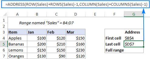
This time, we need a bit more complex calculations to work out the row number. Like in the previous example, the ROW function gives us an array of all the row numbers in the range, {4;5;6;7} in our case. We need to "shift" these numbers by the total row count minus 1, so that the first item in the array becomes the last row number. To find the total row count, we employ the ROWS function and subtract 1 from its result: (4-1=3). Then, we add 3 to each element of the initial array to do the required shift: {4;5;6;7} + 3 = {7;8;9;10}.
The column number is calculated in a similar manner: {2,3,4}+3-1 = {4,5,6}
From the above arrays of row and column numbers, the ADDRESS function assembles an array of cell addresses, but returns only the first one corresponding to the last cell in the range.
The same result can also be achieved by picking the maximum values from the arrays of the row and column numbers. However, this only works in an array formula, which requires pressing Ctrl + Shift + Enter to be completed correctly:
=ADDRESS(MAX(ROW(Sales)), MAX(COLUMN(Sales)))
How to get full address of a named range
To return the complete address of a named range, you just need to concatenate the two formulas from the previous examples and insert the range operator (:) in-between.
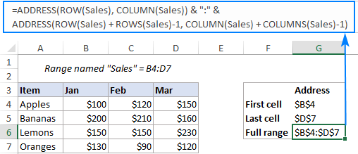
To make it work for our sample data set, we replace the generic "range" with the real range name "Sales":
=ADDRESS(ROW(Sales), COLUMN(Sales)) & ":" & ADDRESS(ROW(Sales) + ROWS(Sales)-1, COLUMN(Sales) + COLUMNS(Sales)-1)
And get the complete range address as an absolute reference $B$4:$D$7:
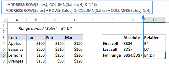
To return the range address as a relative reference (without the $ sign, like B4:D7), set the abs_num argument in both ADDRESS functions to 4:
=ADDRESS(ROW(Sales), COLUMN(Sales), 4) & ":" & ADDRESS(ROW(Sales) + ROWS(Sales)-1, COLUMN(Sales) + COLUMNS(Sales)-1, 4)
Naturally, the same changes can be made in individual formulas for the first and last cell, and the result will look similar to this:
How to get the address of a named range in Excel 365 and Excel 2021
Unlike the traditional "one formula - one cell" behavior in older versions, in new Excel, any formula that can potentially return multiple values, does this automatically. Such behavior is called spilling.
For example, instead of returning the address of the first cell, the below formula outputs the addresses of each and every cell in a named range:
=ADDRESS(ROW(Sales), COLUMN(Sales))
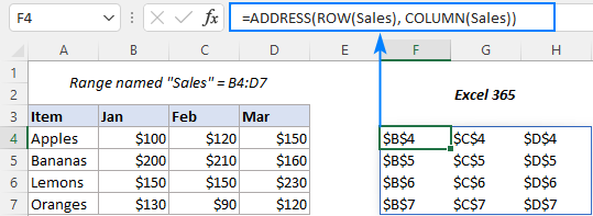
To get the address of the first cell only, you need to enable implicit intersection, which is triggered by default in Excel 2019 and older. For this, put the @ symbol (implicit intersection operator) before the range names:
=ADDRESS(@ROW(Sales), @COLUMN(Sales))
In a similar manner, you can fix other formulas.
To get last cell in the range:
=ADDRESS(@ROW(Sales) + ROWS(Sales)-1, @COLUMN(Sales) + COLUMNS(Sales)-1)
To get the address of a named range:
=ADDRESS(@ROW(Sales), @COLUMN(Sales)) & ":" & ADDRESS(@ROW(Sales) + ROWS(Sales)-1, @COLUMN(Sales) + COLUMNS(Sales)-1)
The below screenshot shows the results:
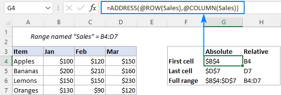
Tip. When opening a worksheet with formulas created in an older version in dynamic array Excel, an implicit intersection operator is inserted by Excel automatically.
That's how you return a cell address in Excel. To have closer look at all the formulas discussed in this tutorial, you are welcome to download our sample workbook below. I thank you for reading and hope to see you on our blog next week!
Practice workbook for download
Excel ADDRESS function - formula examples (.xlsx file)
 by
by
66 comments
hi if i have a list of addresses in a column (all of H) and different names corresponding to these addresses in another column (all of B) is there a way to find any matching addresses in column H and them it pull the corresponding name from column b even if this is different name and produce these into na table?
column b column h
john smith 1 abc close
joe bloggs 3 dfg close
joe smith 3 dfg close
joe smith 1 abc close
joe bloggs 1 abc close
john bloggs 5 ghj close
1 abc close 3 dfg close 5ghj close
john smith joe bloggs john bloggs
joe smith joe smith
joe bloggs
something like the above if that helps with the explanation thanks
Hello! If I understand your task correctly, the following tutorial should help: Vlookup to return multiple matches in rows.
I have a Sheet of different names and items with their receiving is issuing dates. i want to make another sheet of every single item with all their details.
Hi! If I understand your task correctly, try to use FILTER function. Read more: Excel FILTER function - dynamic filtering with formulas.
I know the address of a cell. How can I change the value of it by its address?
For example, there is no value at address A6 and I am trying to enter the value of cell(B6) in a different worksheet.
Is it possible: function(A6, B6) so that the value at address B6 updates the value in cell A6.
Hi! You can update the value of a cell with an external reference. Write in A6: =Sheet1!B6. Read more here: Excel reference to another sheet or workbook (external reference).
Thank you so much for this instruction! How can this be tailored for removing rows from a table? The rows are removed from the main table and placed in a separate table once the item is complete. My formula returns results based off the month (columns E-P) that have both N/A and 0 as entries. My current formula looks like this:
=CHOOSECOLS(FILTER(Table1, (INDIRECT("'Current Checklist'!"&ADDRESS(3,MATCH(E$3,'Current Checklist'!$A$2:$Q$2,0))&":"&ADDRESS(52,MATCH(E$3,'Current Checklist'!$A$2:$Q$2,0))) = 'Current Checklist'!T3),"No data"),1,2,3,4,MATCH(E3,'Current Checklist'!$A$2:$Q$2,0))
The issue becomes when I delete the row as mentioned, the formula breaks until I update the second ADDRESS row number from 52 to whatever the new row number is after deletion. Nothing else in this formula changes. Is there a way I can update the Address formula for this?
I have multiple columns and have just one row. I need to locate the address of the column for a specific text. Could you please help me with that? Thank you.
Hello!
If I understand you correctly, first find a text match using the SEARCH function. The MATCH function will determine the number of that cell in the range. The OFFSET function will move to that cell. The CELL function will find its address. Here is an example of a formula:
=CELL("address",OFFSET(A1,0, MATCH(TRUE, ISNUMBER(SEARCH("abc",A1:E1)),0))
Hope this is what you need.
I am interested in get the address of min value of cell within specify RANGE . I broke my head. Thank you.
Hello!
Write this formula on the first row of your worksheet
=ADDRESS(MATCH(MAX(A1:A100),A1:A100,0),1,1)
This should solve your task.
Hi, I´d like to know how to use Address function as an argument in others functions which use intervals like COUNT, COUNTIF, COUNTA
Hi!
Unfortunately, these functions only need to use ranges of values and must be specified explicitly.
i have a range defined as the Selection.CurrentRegion.Select
in this range are 3 cells.
2 colored green #99FF99 and 1 colored blue #00FFFF
i don't know the best approach to this
any guidance is appreciated
it seems some of my message was deleted
should read:
i have a range defined as the Selection.CurrentRegion.Select
in this range are 3 cells.
2 colored green #99FF99 and 1 colored blue #00FFFF
I simply want created a macro to find these and copy each of these 3 cells to the one below
i don't know the best approach to this
any guidance is appreciated
Hi!
Sorry, we don't provide help with Excel macro and VBA code.
Hello, I have a rather tricky problem and I'm not sure if its possible on Excel.
I have the cell address of a client with the different projects listed in the column to the right hand side. There are a different number of projects for each client. I am after a way of creating an address range for the list of projects. Example below
A B
Nike Shoes
Tops
Shorts
Adidas Shoes
Hats
Is there a way of scanning across from A1 where the Client name is located and returning the cell address B1:B3 or however many projects there are? Might it help if I placed something in the gap between the two project lists.
This is the last piece of the puzzle in my spreadsheet if anyone could point me in the right direction I would be grateful.
Many thanks in advance,
Martin
A................................B
Nike..........................Shoes
..................................Tops
..................................Shorts
............................................
Adidas.....................Shoes
..................................Hats
Hello!
Unfortunately, I cannot help solve your problem with native Excel formulas.
Hi, I want to search a column on another sheet for a name and then return the address the name is in. How would I do this?
Many thanks in advance.
Hello!
To find the value and return the address of an Excel cell, use the CELL function.
Here's an example:
=CELL("address",INDEX(A1:A10,MATCH("aaa",A1:A10,0)))
I hope this will help
Worked a treat! Big thank you
Hi,
I have a similar issue which this formula is close to solving after trying it but with one exception:
When searching the array for the match, I would like it to return each entry as there may be multiple which aren't exact matches.
Is this possible?
Thankyou
Hi! CELL function can return the address of only one cell. Also INDEX+MATCH can return only one value.
Hi, I was trying to this section "How to get address of the first cell in a range"
ADDRESS(ROW(range),COLUMN(range))
But Excel returned an array instead of the first cell address, any idea?
Thanks in advance
Hi!
The information you provided is not enough to understand your case and give you any advice.
What formula did you use and what result did you get?
Hi Alexander,
Thanks for your reply, I was using ADDRESS(ROW(range),COLUMN(range)). My table range start from B2:C7.
So if I am using ADDRESS(ROW(range),COLUMN(range), it should return as first cell which is B2, right? But I am getting the entire table as array showing the cell address
B2 C2
B3 C3
B4 C4
B5 C5
B6 C6
B7 C7
Hello!
I am assuming you are using OFFICE365. At the time of this article writing, it didn't exist yet. This formula should be written as
=ADDRESS(@ROW(Sales),@COLUMN(Sales))
You can download Excel ADDRESS Function Sample Workbook.
We will also definitely update the article.
Hi Shau,
For the formula to work correctly in Excel 365, you need to put @ (implicit intersection operator) before the range names as Alexander suggested. I have added an separate example explaining this in more detail, please see:
How to get the address of a named range in Excel 365
Hi,
If i wanted to find Building name from address mentioned in single cell then which formula should i use & how to use. Also, i have more than 8000 entries & building name differs in all of them.
e.g if i want to find- SAI GHARKUL from
PLOT A- 4A, A- 4B ,B/ H DHOOT HOSPITAL ,FLAT NO 6 Plot No- A- 4( A) A- 4( B) Gut No- 32/ 2 Brijwadi Chikalthana MIDC Aurangabad ,SAI GHARKUL ,Aurangabad (MH) H.O, AURANGABAD-MH, MAHARASHTRA, INDIA - 431001
Thanks in advance.
Hello!
I didn't quite understand what you want to find. But if you need to find text in a cell, use the SEARCH function.
I want to row number and column number of maximum value in a table of ten day sales of ten members..........like table adress a2:k10... acolumn contain name...so data set is b2:k10....from this set i want maximum value row and column number or cell address...please can anyone told me how to find it
Really stuck. I have a worksheet that is dynamic In that I add data each day in a new row. Column A are dates. Column E includes cells where data appears if it meets criteria. For example if D4 is more than 6% Place percent in E4. I then want to look forward x number of days to see what happens on the value.
I need to write various calculations for column E such as sum, count, average etc. the problem is I need to back up the number of days in the column. Example: =SUM(E5:last cell minus the number of days)
The number of days would be in a absolute reference cell that I can change. Maybe 5 days, maybe 10 days etc.
I can write a formula to reference the last cell in column A (the date column that always has data)
=ADDRESS(MATCH(9.99999999999999E+307,A:A),1,3)
This returns for Example $A5627
I now need to offset that result to Column E but also offset back up the number of rows defined in the days selected. For example, if the number of days I want is 10 I would need the result to be $E5617.
That formula would then be nested in my calculations. Example: =Sum(E5:The offset address formula you help me write)
In summary. Find the last row using the date column A which always has data, then offset to Column E backing up rows defined in my number of days reference cell. That formula will return a reference that will then be used in a calculation. Example: =SUM(E5:the formula reference you help me write)
Thanks for your time.
Hello!
If the values in column A are entered from the first row, then the number of the last row with data can be calculated using the formula
=COUNTA(A1:A200)
If I understood the problem correctly, then the formula for the sum
=SUM(INDIRECT("E1:E"&COUNTA(A1:A200)))
Thank you for taking the time to reply. I really appreciate that. I think the formula you replied with would tell me the right row number for the last entry in column E but it still would not offset it by the number of days chosen. I guess I did not explain myself well which was my fear.
For some reason after contemplating this for the last 4 days and hours searching the Internet the solution popped in my head when I woke up today. I merely changed my formula to a IF OR statement that basically looked to see if there was data say 10 days after an entry and it would display the result and if not then it wouldn’t. Problem solved.
Again, thanks for your time.
How to indirect addresses that are not continuous:
=INDIRECT({"$M$2";"$N$2";"$O$2";"$P$2";"$Q$2";"$R$2"}) ””
F9:{"test5";#VALUE!;"test6";"";0;0} ””
F9:{#VALUE!;#VALUE!;#VALUE!;#VALUE!;#VALUE!;#VALUE!})
I expect
={FALSE;#VALUE!;FALSE;TRUE;FALSE;FALSE}
Thanks Ahead
This means that if some rows in a database have a * mark in a specific field, how can the address of all these rows be returned? For example, if we have a * sign in the addresses A1: A3 and A5: A10, how can we return the address of column B in the addresses B1: B3 and B5: B10.
Hello!
I don't quite understand what result you want to get. To determine if there is an "*" character in a cell, you can use the formula:
=ISNUMBER(SEARCH("~*",A2,1))
For me to be able to help you better, please describe your task in more detail.
Is it possible Excel 365 formula to indirect array of columns ={10,12,14} same row? Thanks Ahead!
Last try!
12 13 14 15 16 17 18 19 20
W1 6 6 5 9 16
W2 6 8 7 7 5 12 11 9
W3 9 4 10 5 8 5 1 3 4
W4 10 9 7 8 5 7 4
W5 7 11 6 4 12 8
W6 9 6 5 6 2
Sorry Alexander. Hope this makes more sense as a dataset.
12 13 14 15 16 17 18 19 20
W1 6 6 5 9 16
W2 6 8 7 7 5 12 11 9
W3 9 4 10 5 8 5 13 4
W4 10 9 7 8 5 7 4
W5 7 11 6 4 12 8
W6 9 6 5 6 2
Hi Alexander
This is a small example of the dataset. At the top, the numbers 11 to 20 are the 'Header'. On the left are the row identifiers.
I want to be able to retrieve the top 10 highest numbers i the data set, with their Row ID and Header value.
For example, the ranked (large1) answer would be: "16" "W1" "18" The problem is, when duplicate numbers appear, eg the 2nd highest value is "12". I want to retrieve this as "12" "W2" "17" but also "12" "W5" "18". The solution would look like -
Rank Number Row Header
1 16 W1 18
2 12 W2 17
3 12 W5 18
12 13 14 15 16 17 18 19 20
W1 6 6 5 9 16 6
W2 6 8 7 7 5 12 7 11 9
W3 9 4 10 5 8 5 13 4
W4 10 9 7 8 5 7 4
W5 7 11 6 4 12 8
W6 9 6 5 6 2
I hope this helps....
Tom
I have a 50 X 50 data set of numbers, with duplicates and blanks. I have a header row of letters and a numerical row to the left of the set. I want a formula to be able to retrieve the left number and the appropriate header letter of (for example) the top 10 values in the set. I need the formula to report different addresses for duplicate values in the set.
If it's too complicated, 2 different formulas to report the letter and the number separately would be ok.
Is this possible?
Hi, I have data that is enetered on sheet 1 and have selected a range of that data that is important to automatically appear on sheet2. I would then like to have that data on sheet2 which is in cell E27, search a given range A1 to H22 for a match and provide me with the cell reference of that match. Is this possible?
Any help you can provide would be fantastic, thank you.
I have a partial text in same column multiple times & require to retrieve row number of each.
Formula. =MATCH(DG5&”*”,$AK:$AK,0)*1 Returns 27 Exact match
When I copy down *2 it returns 54 which isn’t a match as it multiply first row number by 2.
DG = partial text
AK:AK. = column reference
Regards
Tony
Hello!
Sorry, it's not quite clear what you are trying to achieve. Without seeing your data it is difficult to give you any advice. Could you please describe it in more detail? Why are you multiplying the formula by 2?
Hi Alexander
I don’t won’t to multiply, need to find row number of each partial text in the same column, the formula =MATCH(DG5&”*”,$AK$AK,0)
How do I change the formula to return row number 1st partial text, 2nd partial text, 3rd partial text & so on in same column?
Regards
Tony
Hi Alexander
Sent a sample excel sheet for your review.
Regards
Tony
I am trying to compare two colums and get the cell address. for example if column 1 has a match in column 2 what is the cell address of the match in column 2
Hello!
Please check out the following article on our blog, it’ll be sure to help you with your task: Compare 2 columns to find duplicates using Excel formulas
I believe the following formula will help you solve your task:
=IF(ISERROR(MATCH(A1,$B$1:$B$10000,0)),"Unique",ADDRESS(MATCH(A1,$B$1:$B$10000,0),2))
I hope I answered your question. If something is still unclear, please feel free to ask.
Svetlana,
Thank you. This is exactly what I was looking for after about searching through 20 articles, and to evaluate a short column of positive nonzero integers.
=MODE(B13:INDIRECT(B5)) Where B5 contains =ADDRESS(COUNTIF(B13:B1000,">0")+ROW(B12),2,4)
And where B13 is the first cell in the data, and the last cell is calculated by the ADDRESS function.
This is also the first time I used a formula in the ":" range syntax as shown.
I am trying to figure out which functions to use to find ”number of people attending”, from a column with blank cells and zeros. However I have the cost of each invitation, tax, and the amount it adds up to. Help!
Hello!
Your question is not related to using the ADDRESS function. I recommend that you study this guide on counting the number of values and, if necessary, ask your question there.
Hi, I am trying to increment the row number of the value of a cell. This value references another workbook.
The formula in cell A1 which gives me the absolute address from the other workbook is =CELL("ADDRESS",INDEX('[WORKBOOKNAME.XLS]WORKSHEETNAME'!$A:$A,MATCH("*WA(*",'[WORKBOOKNAME.XLS]WORKSHEETNAME'!$A:$A,0)))
The value of this results in:
'[WORKBOOKNAME.XLS]WORKSHEETNAME'!$A:$251
I now want to use this address in another formula but increment by 1 for each row it is used in
Is this possible, many thanks
Hello!
I’m sorry but your task is not entirely clear to me.
$A:$251 - this link is not possible.
Write down exactly what you are getting now and what you want to get when you move to the next line. Describe your problem in more detail.
Ultimately I want to use the cell address of a cell from another workbook.
In order to do this I search a column in the different workbook for a matching string and return its cell address;
=CELL("ADDRESS",INDEX('[WORKBOOKNAME.XLS]WORKSHEETNAME'!$A:$A,MATCH("*WA(*",'[WORKBOOKNAME.XLS]WORKSHEETNAME'!$A:$A,0)))
this works and gives me a result in cell A1 of...
'[WORKBOOKNAME.XLS]WORKSHEETNAME'!$A:$251
I then want to use this cell address in another formula to retrieve the value of the cells and offset cells in the other workbook.
I don't want to use VBA.
=ADDRESS(MATCH('ROOM1'!$Q$11'ROLL NUMBERS'!A:A,0)+1,1) NOT GETTING REFRENCE OF SECOND SHEET FROM SHEET 1
Hello!
I cannot validate the formula on your data. But something like this will work for you
=ADDRESS(MATCH(Sheet6!Q11,Sheet16!A:A,0)+1,1)
Hope this is what you need.
I am trying to get the string from cell address.
something that does this: =SomeFormula(A1) returns A1 as string.
thank you in advance.
Hello!
If I understand your task correctly, the following formula should work for you:
=ADDRESS(ROW(),COLUMN(),4,1)
I have such SUMIFS formula working fine:
=SUMIFS('Taches Dev'!V3:V$1000,'Taches Dev'!B$3:B$1000,A2,'Taches Dev'!C$3:C$1000,L$1)
where
'Taches Dev'!V3:V$1000 is my sum range.
In another 2 cells, I have formulas returning the adresses of the two bounds of my range
=ADRESSE(3;EQUIV(M1;'Taches Dev'!A2:AI2;0);;;"Taches Dev") --> Taches Dev'!V3
=ADRESSE(1000;EQUIV(M1;'Taches Dev'!A2:AI2;0);;;) --> V$1000
I'd like to use directly these 2 formulas into the SUMIFS function for determining my sum range.
But I'm getting an error.
Any idea?
Many Thanks in advance
Hello Remy!
To specify a range of cells, you can use the following formula:
INDIRECT(B21&":"&B23)
About the INDIRECT function read the instructions on our blog.
I hope this will help, otherwise please do not hesitate to contact me anytime.
is there any function in excel that finds the requied value in a range and returns Left most column value and top most row value in that range for the found cell.
is there any function in excel that finds the requied value in a range and returns Left most column value and top most row value in that range for the found cell.
Hi Svetlana Cheusheva. I have this formula:
=CELL("address";INDEX(Sheet2!A2:D5;MATCH(Sheet1!A1;Sheet2!D2:D5;0);4;1))
That returns:
'[Book1 (version 1).xlsb]Sheet2'!$D$1
How to show not the file name?
I’m trying to find the address of the First five row numbers in a given column where continuously the cell values are >= X, There can be multiple instances where we can find the continuous rows where cell values are >=X, but I need to find the first occurrence only.
For example in column A, continuously values in the 5 rows i.e., A6 A7 A8 A9 A10 are >=x and also in row number A15 A16 A17 A18 A19, etc.
The row# A6 to A10 is the first occurrence (first five consecutive values) and I need the address of the row numbers as output i.e., A6: A10