The tutorial shows how to use the SORT function to sort data arrays dynamically. You will learn a formula to sort alphabetically in Excel, arrange numbers in ascending or descending order, sort by multiple columns, and more.
The Sort functionality has been around for a long time. But with the introduction of dynamic arrays in Excel 365, there appeared an amazingly simple way to sort with formulas. The beauty of this method is that the results update automatically when the source data changes.
Excel SORT function
The SORT function in Excel sorts the contents of an array or range by columns or rows, in ascending or descending order.
SORT belongs to the group of Dynamic array functions. The result is a dynamic array that automatically spills to neighboring cells vertically or horizontally, depending on the shape of the source array.
The syntax of the SORT function is as follows:
Where:
Array (required) - is an array of values or a range of cells to sort. These can be any values including text, numbers, dates, times, etc.
Sort_index (optional) - an integer that indicates which column or row to sort by. If omitted, the default index 1 is used.
Sort_order (optional) - defines the sort order:
- 1 or omitted (default) - ascending order, i.e. from smallest to largest
- -1 - descending order, i.e. from largest to smallest
By_col (optional) - a logical value that indicates the direction of sorting:
- FALSE or omitted (default) - sort by row. You'll use this option most of the time.
- TRUE - sort by column. Use this option if your data is organized horizontally in columns like in this example.
Excel SORT function - tips and notes
SORT is a new dynamic array function and as such it has a couple of specificities that you should be aware of:
- Currently the SORT function is only available in Microsoft 365 and Excel 2021. Excel 2019, Excel 2016 do not support dynamic array formulas, so the SORT function is not available in these versions.
- If the array returned by a SORT formula is the final result (i.e. not passed to another function), Excel dynamically creates an appropriately sized range and populates it with the sorted values. So, be sure you always have enough empty cells down or/and to the right of the cell where you enter the formula, otherwise a #SPILL error occurs.
- The results update dynamically as the source data changes. However, the array supplied to the formula does not extend automatically to include new entries that are added outside of the referenced array. To include such items, you need to either update the array reference in your formula, or convert the source range to an table as shown in this example, or create a dynamic named range.
Basic Excel SORT formula
This example shows a basic formula for sorting data in Excel in ascending and descending order.
Supposing your data is arranged alphabetically as shown in the screenshot below. You are looking to sort numbers in column B without breaking or mixing data.
Formula to sort in ascending order
To sort values in column B from smallest to largest, here's the formula to use:
=SORT(A2:B8, 2, 1)
Where:
- A2:B8 is the source array
- 2 is the column number to sort by
- 1 is the ascending sort order
Since our data is organized in rows, the last argument can be omitted to default to FALSE - sort by rows.
Just enter the formula in any empty cell (D2 in our case), press Enter, and the results will spill automatically to D2:E8.
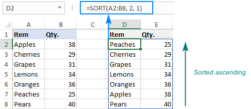
Formula to sort in descending order
To sort data descending, i.e. from largest to smallest, set the sort_order argument to -1 like this:
=SORT(A2:B8, 2, -1)
Enter the formula in the top left cell of the destination range and you will get this result:
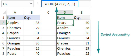
In a similar manner, you can sort text values in alphabetical order from A to Z or from Z to A.
How to sort data in Excel using formula
The below examples show a few typical uses of the SORT function in Excel and a couple of non-trivial ones.
Excel SORT by column
When you sort data in Excel, for the most part you change the order of rows. But when your data is organized horizontally with rows containing labels and columns containing records, you might need to sort from left to right, rather than from top to bottom.
To sort by column in Excel, set the by_col argument to TRUE. In this case, sort_index will represent a row, not a column.
For example, to sort the below data by Qty. from highest to lowest, use this formula:
=SORT(B1:H2, 2, 1, TRUE)
Where:
- B1:H2 is the source data to sort
- 2 is the sort index, since we are sorting numbers in the second row
- -1 indicates the descending sort order
- TRUE means to sort columns, not rows

Sort by multiple columns in different order (multi-level sort)
When working with complex data models, you may often need a multi-level sort. Can that be done with a formula? Yep, easily! What you do is to supply array constants for the sort_index and sort_order arguments.
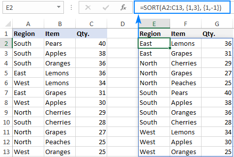
For example, to sort the below data first by Region (column A) from A to Z, and then by Qty. (column C) from smallest to largest, set the following arguments:
- Array is the data in A2:C13.
- Sort_index is the array constant {1,3}, since we first sort by Region (1st column), and then by Qty. (3rd column).
- Sort_order is the array constant {1,-1}, since the 1st column is to be sorted in ascending order and the 3rd column in descending order.
- By_col is omitted because we sort rows, which is default.
Putting the arguments together, we get this formula:
=SORT(A2:C13, {1,3}, {1,-1})
And it works perfectly! The text values in the first column are sorted alphabetically and the numbers in the third column from largest to smallest:
Sort and filter in Excel
In case when you are looking to filter data with some criteria and put the output in order, use the SORT and FILTER functions together:
The FILTER function gets an array of values based on the criteria you define and passes that array to the first argument of SORT.
The best thing about this formula is that it also outputs the results as a dynamic spill range, without you having to press Ctrl + Shift + Enter or guess at how many cells to copy it to. As usual, you type a formula in the upper most cell and hit the Enter key.
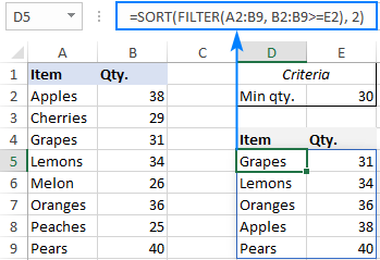
As an example, we are going to extract items with quantity equal to or greater than 30 (>=30) from the source data in A2:B9 and arrange the results in ascending order.
For this, we first set up the condition, say, in cell E2 as shown in the image below. And then, build our Excel SORT formula in this way:
=SORT(FILTER(A2:B9, B2:B9>=E2), 2)
Apart from array generated by the FILTER function, we only specify the sort_index argument (column 2). The remaining two arguments are omitted because the defaults work exactly as we need (sort ascending, by row).
Get N largest or smallest values and sort the results
When analyzing huge bulks if information, there is often a need to extract a certain number of top values. Maybe not just extract, but also arrange them in the desired order. And ideally, choose which columns to include in the results. Sounds tricky? Not with the new dynamic array functions!
Here is a generic formula:
Where n is the number of the values you want to return.
From the below data set, assume you want to get a top 3 list based on the numbers in column C.
To have it done, you first sort the array A2:C13 by the 3rd column in descending order:
SORT(A2:C13, 3, -1)
And then, nest the above formula in the first (array) argument of the INDEX function to have the array sorted from highest to smallest.
For the second (row_num) argument, which indicates how many rows to return, generate the required sequential numbers by using the SEQUENCE function. As we need 3 top values, we use SEQUENCE(3), which is the same as supplying a vertical array constant {1;2;3} directly in the formula.
For the third (col_num) argument, which defines how many columns to return, supply the column numbers in the form of a horizontal array constant. We want to return columns B and C, so we use the array {2,3}.
Eventually, we get the following formula:
=INDEX(SORT(A2:C13, 3, -1), SEQUENCE(3), {2,3})
And it produces exactly the results we want:
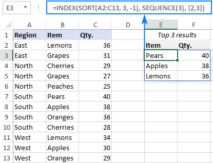
To return 3 bottom values, simply sort the original data from smallest to largest. For this, change the sort_order argument from -1 to 1:
=INDEX(SORT(A2:C13, 3, 1), SEQUENCE(3), {2,3})
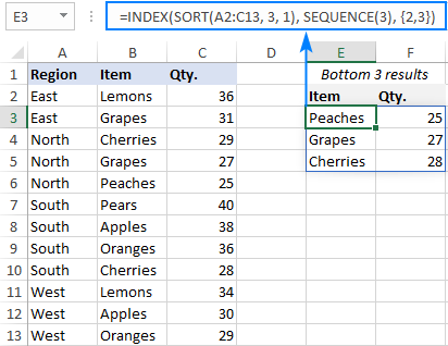
Return a sorted value in a specific position
Looking from another angle, what if you only want to return a specific sort position? Say, only the 1st , only the 2nd, or only the 3rd record from the sorted list? To have it done, use the simplified version of the INDEX SORT formula discussed above:
Where n is the position of interest.
For example, to get a particular position from top (i.e. from the data sorted descending), use this formula:
=INDEX(SORT(A2:C13, 3, -1), F1, {2,3})
To get a specific position from bottom (i.e. from the data sorted ascending), use this one:
=INDEX(SORT(A2:C13, 3, 1), I1, {2,3})
Where A2:C13 is source data, F1 is the position from top, I1 is the position from bottom, and {2,3} are the columns to be returned.
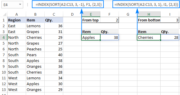
Use Excel table to get sort array to expand automatically
As you already know, the sorted array updates automatically when you make any changes to the original data. This is the standard behavior of all dynamic array functions, including SORT. However, when you add new entries outside the referenced array, they are not automatically included in a formula. If you'd like your formula to respond to such changes, convert the source range to a fully-functional Excel table and use structured references in your formula.
To see how it works in practice, please consider the following example.
Supposing you use the below Excel SORT formula to arrange values in the range A2:B8 in alphabetical order:
=SORT(A2:B8, 1, 1)
Then, you input a new entry in row 9… and are disappointed to see that the newly added entry is left out of the spill range:
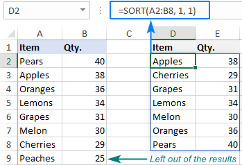
Now, convert the source range to a table. For this, simply select your range including the column headers (A1:B8) and press Ctrl + T. When building your formula, select the source range using the mouse, and the table name will be inserted in the formula automatically (this is called a structured reference):
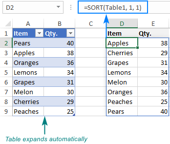
=SORT(Table1, 1, 1)
When you type a new entry right below the last row, the table will expand automatically, and the new data will be included in the spill range of the SORT formula:
Excel SORT function not working
If your SORT formula results in an error, it's most likely because of the following reasons.
#NAME error: older Excel version
SORT is a new function and works only in Excel 365 and Excel 2021. In older versions where this function is not supported, a #NAME? error occurs.
#SPILL error: something blocks spill range
If one or more cells in the spill range are not completely blank or merged, a #SPILL! error is displayed. To fix it, just remove the blockage. For more information, please see Excel #SPILL! error - what it means and how to fix.
#VALUE error: invalid arguments
Whenever you run into a #VALUE! error, check the sort_index and sort_order arguments. Sort_index should not exceed the number of columns is array, and sort_order should be either 1 (ascending) or -1 (descending).
#REF error: source workbook is closed
Since dynamic arrays have limited support for references between workbooks, the SORT function requires both files to be open. If the source workbook is closed, a formula will throw a #REF! error. To fix it, just open the referenced file.
That's how to sort data in Excel using formula. I thank you for reading and hope to see you on our blog next week!
Practice workbook for download
Sorting in Excel with formulas (.xlsx file)
 by
by
53 comments
hi, I am looking at a time series of (daily) stock prices with Date (in Column A); High (Col B); Low (Col C); Close (Col D), Volume (Col E), and Remarks (Col F) with 'R','S' or empty as entries. Expectedly, row 1 are the 'Labels' above, e.g. cell B1 is 'High'.
If I would like to arrange the stock prices in descending order (say in Column H), with Col I indicating whether it is a 'High', 'Low' or 'Close', Col J indicating 'Volume', and Col K indicating 'Remarks' ('R','S' or empty). How should I go about it please? (Certainly, the same prices may occur few times under different columns). Thanks!
Hi! Your request goes beyond the advice we provide on this blog. This is a complex solution that cannot be found with a single formula. If you have a specific question about the operation of a function or formula, I will try to answer it.
I am doing a time off request log. I am trying to sort the table by the drop down options. For example, Submitted, Denied, Approved. These are drop downs in my column B. I would like the table to sort Submitted at the top, Then Denied, Then Approved automatically. (Ideally, I would have like them to sort to new headers underneath with the same names) But I will take them just sorting in order of option selected.
Hi! You can use the SORT formula for sorting as described in the article above. This guide may also be helpful: How to sort in Excel by row, column names and in custom order.
=LET(
a,FILTER(CHOOSE({1,2,3,4,5,6,7,8},INDIRECT($B$1&"!$A$4:$a$11000"),INDIRECT($B$1&"!$b$4:$b$11000"),INDIRECT($B$1&"!$e$4:$e$11000"),INDIRECT($B$1&"!$f$4:$f$11000"),INDIRECT($B$1&"!$g$4:$g$11000"),INDIRECT($B$1&"!$h$4:$h$11000"),INDIRECT($B$1&"!$i$4:$i$11000"),INDIRECT($B$1&"!$k$4:$K$11000")),((IF(K2="",TRUE,INDIRECT($B$1&"!$A$4:$A$11000")=K2))*(INDIRECT($B$1&"!$e$4:$e$11000")""))+(ROW(INDIRECT($B$1&"!$A$4:$A$11000"))=4)),
IFERROR(SORTBY(a,MATCH(INDEX(a,,1),Customlist!$B$1:$B$5,0),1,INDEX(a,,5),1,INDEX(a,,2),1),"Not found")).
Can you make it short this formula as it is too lengthy.
It is very difficult to understand a formula that contains unique references to your workbook worksheets.
I can share the file via email.Cannot do in public.If u do not mind,how to connect by email.
Taking whole data in formula but offsetting row 1 which is header.How,this can be done ?
What formula are you talking about? If you want help, ask the right question.
I use the following formula to find names of people that correspond with the word "Shop" in a table. Is there a way to ad additional text values to search for within this formula? So, it would search for "Shop" or "Home" or "Work" for example.
=FILTER(B71:B110,ISNUMBER(SEARCH("Shop",Table2[Area])))
Hi!
You can add several conditions to the FILTER function as described in this article: Filter with multiple criteria (OR logic).
=FILTER(B71:B110,ISNUMBER(SEARCH("Shop",Table2[Area]))+ISNUMBER(SEARCH("Home",Table2[Area])))
Sorting based on a column that contains a formula (resulting a numeric value) does not work. Any clue how should I make it work?
Hello,
This issue was due to the fact, the columns were part of separate table in excel. Making the formula column part of the same table, solved the issue.
Hi!
It seems that "-1" in =SORT(A2:B8, 2, -1) is not working in google sheets. I want it to be descending, but it keeps coming ascending.
Any suggestions, please?
Thanks!
Hi!
In the SORT function of Google Sheets, the sort order is defined as TRUE and FALSE
Dear Alexander,
Thanks for the response!
I have tried TRUE and FALSE, but still I couldn't make it work.
Anyway, I came up with this idea: I created an extra column that had the amounts in negative form, and I used that column as a criterion for sorting. Then I hid that extra column, so now I have the chart as I wanted it, amounts in descenting order!
How about that!
Thanks!
if my colum looks like:
A 12
B 3
C 34
D 64
E 325
And i want to sort by number (descending)
and my formula looks like:
=SORT((A2:B15;B2:B15;-1;False)
it gives the error value
Hi!
Take a look at the SORT function syntax. The [sort_index] argument is not a range, but a column number.
=SORT((A2:B15;2;-1;False)
I want to arrange the column B as per the order of Column A using sort formula is it possible do such a sorting in Excel
Hi! Try to use the recommendations described in this article: Excel SORTBY function - custom sort with formula.
You can also sort the table by column A without formula using Excel tools. Read more: How to sort in Excel by row, column names and in custom order.
hello!
I have a table with two columns:
France 2
Italy 4
Germany 3
I want to sort this by column 2, but column 2, I need multiplie with 2.
for final ai need this:
France 4
Germany 6
Italy 8
thank you!
Hi!
The following tutorial should help: How to multiply a column by number.
You can read how to sort a column in the article above, as well as in this guide: How to alphabetize in Excel: sort columns and rows.
This should solve your task.
thanks for the reply!
I would like to specify that I have two columns for Country and in another I have numbers.
I would sort by the formula as an example:
=SORTBY(A1:B7; B1:B7; 1)
but I need B1 to multiply it by 2 the same and B2...etc
How can I do that in this formula to multiply (B1:B7*2) with 2?
=SORTBY(A1:B7; (B1:B7)*2; 1) , does not work
Thanks and please excuse my English!
Hi!
Multiplication must be done in a separate column. But multiplying by 2 will not affect sorting in any way.
Hi team
Your articles are so helpful thankyou!!
I am struggling with one of the sort functions. I have all my companies listed according to rank. How do I sort the data so it displays the company according to rank position, with number 1 being at the top then descending numbers?
Please help!!
Thanks in advance
Hi!
Define in a separate column the unique rank of each company. You can see an example in the article - How to rank data in Excel uniquely.
Then you can use the SORT function to sort the list of companies by that column.
I hope I answered your question. If something is still unclear, please feel free to ask.
Hello ;
Your article was excellent.
I enjoyed
Hi Team,
Hope you are well.
I have a sales data sheet and using filter and sort function to bring top 10 values by using large function inside sort and filter function. But problem is some sales are same numbers so it’s brings all top 10 sales which is right but I don’t want to exceed fixed number of columns like I need top10 values in 10 columns if top 10 has Some same sales then it will go 11th Column and after but I want to stop at 10th column. Please advise which function I can use to fix this issue.
Thank you for your help in advance.
Thanks
Razib
Hello!
I can't guess which formula you are using. To get a unique rank for each number you can use this tutorial.
Hope this is what you need.
Thank you so much. It helped and solved the issue.
Thanks
Razib
Kindly, how can I install sort() and filter() functions while I already have office 365 on my machine??
Thanks in advance.
Hi Ahmed,
You do not need to install anything, these functions are included in Excel for Microsoft 365. Just start typing a formula in a cell, and you'll see the function's name in the formula intellisense. They are also available in the Function Library on the Formulas tab.
I already tried to type the formula in the cell but it's not included in the drop list of formulas. that is why I am asking if there is an add-on or specific update to make these formulas visible.
In this case, I can only advise installing the latest Office updates to make sure your Excel is up to date.
Very well explained. Thanks
Hi there,
I am trying to use the sort function in a multi-dependent drop down list that used a dynamic named range.
Named ranged
=OFFSET('User Personas'!$A$2,0,0,COUNTA('User Personas'!$A:$A:'User Personas'!$A:$A),1)
Dada validation
=IF(H256=Lists!$A$2,User_Dyn,IF(H256=Lists!$A$3,Location_Dyn,IF(H256=Lists!$A$4,Vehicle_Dyn,IF(H256=Lists!$A$5,Other_Dyn,0))))
However I can not for the life of me get the drop down list to show alphabetically, and I cannot use macros for the task or sort the original dynamic range within the workbook
Hello!
It is very difficult to understand a formula that contains unique references to your workbook worksheets. Hence, I cannot check its work, sorry.
You made my day! Thanks a lot for the detailed explanation. This made my task easier in my work today.
how can we use this but with dates?
NAME CASTE
A SC
B OBC
C ST
A ST
B SC
D ST
A OBC
B ST
D SC
how can possible ?
firstly SC -> name wise
then ST > name wise
then OBC -> name wise
This a great article and has been invaluable in helping me today. Thank you!
I was trying to make something else work and I hope you could help me with. I have a list that I want to sort but I do not want the two sets of columns as in your first example (set one A2:B8 and set two D2:E8) . I just would like to have one set of columns where the inputs and outputs show dynamically. i.e., as I enter a row of information that row will move to its corresponding row order.
Thank you
Hello!
You can learn more about sorting in Excel in this article on our blog.
I hope my advice will help you solve your task.
Hi dear....
Just wanna say Bravo.....
Regards
Hello,
I can see a huge potential in the SORT function and thank you for explaining it so clearly. I was trying to make something else work and I hope you could help me with. I have a list that I want to sort but I do not want the two sets of columns as in your first example (set one A2:B8 and set two D2:E8) . I just would like to have one set of columns where the inputs and outputs show dynamically. i.e., as I enter a row of information that row will move to its corresponding row order.
Please let me know if it makes sense.
Thank you,
Esteban
fromula for automatically sort a data for values only
You should be able to right-click on a column letter and select "sort" among other column options, but the idiots who created this junk had no common sense.
Hi,
I was getting the same issue as Simon - have since realised I'm using Excel 2016 version. I can't upgrade as I'm using this for work purposes so this is the excel version the business uses. Do you have any suggestions on how to sort data if this function "=SORT" is not available? Frustrating really as this function is exactly what I need! I need data that will auto sort as soon as new data is added. Therefore the Sort button is not useful - and I want to avoid using macros if I can.
Hello!
Please check out the following article on our blog, it’ll be sure to help you with your task: Excel alphabetical order with formulas
I hope it’ll be helpful.
I‘m trying to sort a few cells in a row by using
=sort(C2:F2,1,-1,ture)
"That function isn't valid" came out after the formula input.
Hi Simon,
This may happen if you are trying to use the formula in any version other than Excel 365. Please note that all new dynamic array functions including SORT are only available with Microsoft 365 subscriptions.
Also, please notice that "true" is mistyped in the last argument.
It's great learning new ways to use the dynamic array formulas, thanks for this article.
I do have a question. Is there a way when using SORT and multiple columns (i.e. feeding an array constant to the sort columns) to have the columns being sorted on?
Using your example from the multi-level sort section, hypothetically if I had someone enter numbers in cells H1 and I1, could I have those numbers feed into the creation of an array constant to change which columns are used?
e.g. instead of "=SORT(A2:C13, {1,3}, {1,-1})" something that would work on the lines of "=SORT(A2:C13, {H1,I1}, {1,-1})"
I've tried ways of making that happen, but none are successful. Do you know if it can be done?
Hopefully that makes sense?
Hi Jonathan,
Yes, that makes perfect sense :)
Assuming the numbers are entered in adjacent cells like in your example, you can supply them as a normal range:
=SORT(A2:C13, H1:I1, {1,-1})