The tutorial shows how to use IFERROR in Excel to catch errors and replace them with a blank cell, another value or a custom message. You will learn how to use the IFERROR function with Vlookup and Index Match, and how it compares to IF ISERROR and IFNA.
"Give me the place to stand, and I shall move the earth," Archimedes once said. "Give me a formula, and I shall make it return an error," an Excel user would say. In this tutorial, we won't be looking at how to return errors in Excel, we'd rather learn how to prevent them in order to keep your worksheets clean and your formulas transparent.
Excel IFERROR function - syntax and basic uses
The IFERROR function in Excel is designed to trap and manage errors in formulas and calculations. More specifically, IFERROR checks a formula, and if it evaluates to an error, returns another value you specify; otherwise, returns the result of the formula.
The syntax of the Excel IFERROR function is as follows:
Where:
- Value (required) - what to check for errors. It can be a formula, expression, value, or cell reference.
- Value_if_error (required) - what to return if an error is found. It can be an empty string (blank cell), text message, numeric value, another formula or calculation.
For example, when dividing two columns of numbers, you may get a bunch of different errors if one of the columns contains empty cells, zeros or text.
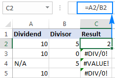
To prevent that from happening, use the IFERROR function to catch and handle errors the way you want.
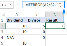
If error, then blank
Supply an empty string (") to the value_if_error argument to return a blank cell if an error is found:
=IFERROR(A2/B2, "")
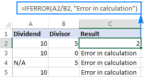
If error, then show a message
You can also display your own message instead of Excel's standard error notation:
=IFERROR(A2/B2, "Error in calculation")
5 things you should know about Excel IFERROR function
- The IFERROR function in Excel handles all error types including #DIV/0!, #N/A, #NAME?, #NULL!, #NUM!, #REF!, and #VALUE!.
- Depending on the contents of the value_if_error argument, IFERROR can replace errors with your custom text message, number, date or logical value, the result of another formula, or an empty string (blank cell).
- If the value argument is a blank cell, it is treated as an empty string (''') but not an error.
- IFERROR was introduced in Excel 2007 and is available in all subsequent versions of Excel 2010, Excel 2013, Excel 2016, Excel 2019, Excel 2021, and Excel 365.
- To trap errors in Excel 2003 and earlier versions, use the ISERROR function in combination with IF, as shown in this example.
IFERROR formula examples
The following examples show how to use IFERROR in Excel in combination with other functions to accomplish more complex tasks.
Excel IFERROR with Vlookup
One of the most common uses of the IFERROR function is telling the users that the value they are searching for does not exist in the data set. For this, you wrap a VLOOKUP formula in IFERROR like this:
If the lookup value is not in the table you are looking in, a regular Vlookup formula would return the #N/A error:
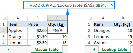
For your users' piece of mind, wrap VLOOKUP in IFERROR and display a more informative and user-friendly message:
=IFERROR(VLOOKUP(A2, 'Lookup table'!$A$2:$B$4, 2,FALSE), "Not found")
The screenshot below shows this Iferror formula in Excel:

If you'd like to trap only #N/A errors but not all errors, use the IFNA function instead of IFERROR.
For more Excel IFERROR VLOOKUP formula examples, please check out these tutorials:
Nested IFERROR functions to do sequential Vlookups in Excel
In situations when you need to perform multiple Vlookups based on whether the previous Vlookup succeeded or failed, you can nest two or more IFERROR functions one into another.
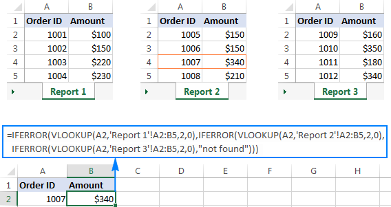
Supposing you have a number of sales reports from regional branches of your company, and you want to get an amount for a certain order ID. With A2 as the lookup value in the current sheet, and A2:B5 as the lookup range in 3 lookup sheets (Report 1, Report 2 and Report 3), the formula goes as follows:
=IFERROR(VLOOKUP(A2,'Report 1'!A2:B5,2,0),IFERROR(VLOOKUP(A2,'Report 2'!A2:B5,2,0),IFERROR(VLOOKUP(A2,'Report 3'!A2:B5,2,0),"not found")))
The result will look something similar to this:
For the detailed explanation of the formula's logic, please see How to do sequential Vlookups in Excel.
IFERROR in array formulas
As you probably know, array formulas in Excel are meant to perform multiple calculations within a single formula. If you supply an array formula or expression that results in an array in the value argument of the IFERROR function, it'd return an array of values for each cell in the specified range. The below example shows the details.
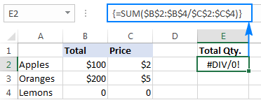
Let's say, you have Total in column B and Price in column C, and you want to calculate Total Quantity. This can be done by using the following array formula, which divides each cell in the range B2:B4 by the corresponding cell of the range C2:C4, and then adds up the results:
=SUM($B$2:$B$4/$C$2:$C$4)
The formula works fine as long as the divisor range does not have zeros or empty cells. If there is at least one 0 value or blank cell, the #DIV/0! error is returned:
To fix that error, simply do the division within the IFERROR function:
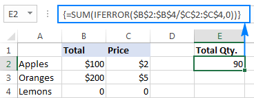
=SUM(IFERROR($B$2:$B$4/$C$2:$C$4,0))
What the formula does is to divide a value in column B by a value in column C in each row (100/2, 200/5 and 0/0) and return the array of results {50; 40; #DIV/0!}. The IFERROR function catches all #DIV/0! errors and replaces them with zeros. And then, the SUM function adds up the values in the resulting array {50; 40; 0} and outputs the final result (50+40=90).
Note. Please remember that array formulas should be completed by pressing the Ctrl + Shift + Enter shortcut.
IFERROR vs. IF ISERROR
Now that you know how easy it is to use the IFERROR function in Excel, you may wonder why some people still lean towards using the IF ISERROR combination. Does it have any advantages compared to IFERROR? None. In the bad old days of Excel 2003 and lower when IFERROR did not exist, IF ISERROR was the only possible way to trap errors. In Excel 2007 and later, it's just a bit more complex way to achieve the same result.
For instance, to catch Vlookup errors, you can use either of the below formulas.
In Excel 2007 - Excel 2016:
In all Excel versions:
Notice that in the IF ISERROR VLOOKUP formula, you have to Vlookup twice. In plain English, the formula can be read as follows: If Vlookup results in error, return "Not found", otherwise output the Vlookup result.
And here is a real-life example of an Excel If Iserror Vlookup formula:
=IF(ISERROR(VLOOKUP(D2, A2:B5,2,FALSE)),"Not found", VLOOKUP(D2, A2:B5,2,FALSE ))

For more information, please see Using ISERROR function in Excel.
IFERROR vs. IFNA
Introduced with Excel 2013, IFNA is one more function to check a formula for errors. Its syntax is similar to that of IFERROR:
In what way is IFNA different from IFERROR? The IFNA function catches only #N/A errors while IFERROR handles all error types.
In which situations you may want to use IFNA? When it is unwise to disguise all errors. For example, when working with important or sensitive data, you may want to be alerted about possible faults in your data set, and standard Excel error messages with the "#" symbol could be vivid visual indicators.
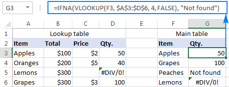
Let's see how you can make a formula that displays the "Not found" message instead of the N/A error, which appears when the lookup value is not present in the data set, but brings other Excel errors to your attention.
Supposing you want to pull Qty. from the lookup table to the summary table as shown in the screenshot below. Using the Excel Iferror Vlookup formula would produce an aesthetically pleasing result, which is technically incorrect because Lemons do exist in the lookup table:
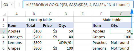
To catch #N/A but display the #DIV/0 error, use the IFNA function in Excel 2013 and Excel 2016:
=IFNA(VLOOKUP(F3,$A$3:$D$6,4,FALSE), "Not found")
Or, the IF ISNA combination in Excel 2010 and earlier versions:
=IF(ISNA(VLOOKUP(F3,$A$3:$D$6,4,FALSE)),"Not found", VLOOKUP(F3,$A$3:$D$6,4,FALSE))
The syntax of the IFNA VLOOKUP and IF ISNA VLOOKUP formulas are similar to that of IFERROR VLOOKUP and IF ISERROR VLOOKUP discussed earlier.
As shown in the screenshot below, the Ifna Vlookup formula returns "Not found" only for the item that is not present in the lookup table (Peaches). For Lemons, it shows #DIV/0! indicating that our lookup table contains a divide by zero error:
For more details, please see Using IFNA function in Excel.
Best practices for using IFERROR in Excel
By now you already know that the IFERROR function is the easiest way to catch errors in Excel and mask them with blank cells, zero values, or custom messages of your own. However, that does not mean you should wrap each and every formula with error handling. The following simple recommendations may help you keep the balance.
- Don't trap errors without a reason.
- Wrap the smallest possible part of a formula in IFERROR.
- To handle only specific errors, use an error handling function with a smaller scope:
- IFNA or IF ISNA to catch only #N/A errors.
- ISERR to catch all errors except for #N/A.
This is how you use the IFERROR function in Excel to trap and handle errors. To have a closer look at the formulas discussed in this tutorial, you are welcome to download our sample IFERROR Excel workbook. I thank you for reading and hope to see you on our blog next week.
 by
by
83 comments
Hello, I will paste my formula below. I am wanting to change the value of #NUM! to blank and am having trouble placing the IFERROR to represent that. Can someone help?
=IF(INT(B22- B20)>0, INT(B22- B20) & " days, ","") & IF(HOUR(B22- B20)>0, HOUR(B22- B20) & " hours, ","") & IF(MINUTE(B22- B20)>0, MINUTE(B22- B20) & " minutes ","")
Hi! All the necessary instructions on how to use the IFERROR function are in the article above. For example:
=IFERROR(IF(INT(B22- B20)>0, INT(B22- B20) & " days, ","") & IF(HOUR(B22- B20)>0, HOUR(B22- B20) & " hours, ","") & IF(MINUTE(B22- B20)>0, MINUTE(B22- B20) & " minutes ",""),"")
Hi What does this means?
=IFERROR(ROUND(AVERAGE(INDIRECT($D6 & $E$4 & F$4):INDIRECT($D6 & $E$4 & F$5)),1),0)
Hi! If you wrote this formula, you must have an idea of what your goal is. You can learn more about INDIRECT function in Excel in this article on our blog: Excel INDIRECT function - basic uses and formula examples.
How to use a sum formula after using lookup in iferror formula?
Unfortunately, this information is not enough to give you any advice.
I have a simple IFERROR formula to calculate a variance% between actuals and budget. Currently, the variance% is showing as a negative value despite actuals outperforming budget.
Example:
Net Income: ($20,000)
Budgeted Net Income: ($30,000)
Variance: +$10,000
Variance%: -33%
*Current formula: =IFERROR(Variance/Budget,"-") results in a negative %. How can I get this to calculate the variance% to be determined by the positive value of the variance amount instead of the mathematical result?
Hi! Your formula and the data you wrote cannot give a negative percent result. 10000/30000=33%. However, you can always apply the ABS function to use the absolute value of the variance.
If I use the ABS function, it will always return a positive result. Correct? I want it to return a negative result when applicable.
I understand from your question that you always want a positive result. I think these instructions will help: How to calculate percentage in Excel - formula examples.
No, I want the sign of the variance% to be determined by the variance amount. If the variance amount is a positive number, I want the variance% to be positive. If the variance amount is negative, I want the variance% to be negative.
In the article I recommended to you, read the paragraph - How to calculate percent difference in Excel.
Hi all, I am looking for a MATCH formula for the following.
SHEET 1: I type a Home# (example Home-1) in column A and a stage (example DRYWALL) in Column B.
Sheet 2: I type a home number again is Column A I would like column B to pull automatically from Sheet one Column B. But it has to match that specific home number.
Reference, I have multiple homes and throughout multiple spreadsheets I update the specific home #’s stage and would like to just update it on sheet 1 and it auto pull onto multiple different sheets.
Hello! You can extract the required value with the VLOOKUP function following these guidelines: Excel VLOOKUP function tutorial with formula examples.
You can also use INDEX+MATCH as described in these instructions: Excel INDEX MATCH vs. VLOOKUP - formula examples.
Hi all,
Does anyone know a formula so it can highlight if a date has changed? I have 2 columns of dates which have hundreds of rows completed and I need a formula to highlight if one of the dates have changed from one column to another. I can then drag this down the rows. My end goal is to give a percentage of dates that have changed
Hi! If I understand your task correctly, this article may be helpful: Compare two columns for matches and differences.
I cannot tell you how helpful this has been. Thank you very much :-)
Hi!
I am comparing the values in two different columns. If the value from column B exists in column A, I want it to say "OLD", but if the value in column B does not exist in column A, I want it to say "NEW". I got it to say "NEW", but for "OLD, it's returning the same name again. How can I customize this second part?
=IFERROR(VLOOKUP(C2,$A$2:$A$1000,1,FALSE),"NEW")
Thank you
Hi! Use the IF function to get "OLD" if VLOOKUP returns a cell value, and get "NEW" if VLOOKUP returns an error.
=IF(ISERROR(VLOOKUP(C2,$A$2:$A$1000,1,FALSE)),"NEW","OLD")
Hi, how to minimize the below formula without changing the result? Thanks.
=IFERROR(IF(DATEDIF(A2,D2,"Y")=0,"",IF(DATEDIF(A2,D2,"Y")>1,DATEDIF(A2,D2,"Y")&" YEARS ",DATEDIF(A2,D2,"Y")&" YEAR "))&IF(DATEDIF(A2,D2,"YM")=0,"",IF(DATEDIF(A2,D2,"YM")>1,DATEDIF(A2,D2,"YM")&" MONTHS ",DATEDIF(A2,D2,"YM")&" MONTH "))&IF(DATEDIF(A2,D2,"MD")=0,"",IF(DATEDIF(A2,D2,"MD")>1,DATEDIF(A2,D2,"MD")&" DAYS ",DATEDIF(A2,D2,"MD")&" DAY ")),"")
Hi! I don't have your data and I can't guess what result you wanted to get
Hi.
I want to ask. How am I supposed to add my arguments, when some of the search that I stated, I wanted it to return to be zero.
=RIGHT(C4,LEN(C4)-(MIN(IFERROR(SEARCH("MXM",C4),9^99),IFERROR(SEARCH("MX7",C4),9^99),IFERROR(SEARCH("MX7",C4),9^99),IFERROR(SEARCH("MX1",C4),9^99),IFERROR(SEARCH("MX2",C4),9^99),IFERROR(SEARCH("MX4",C4),9^99),IFERROR(SEARCH("MX3",C4),9^99),IFERROR(SEARCH("DX",C4),9^99),IFERROR(SEARCH("MX5",C4),9^99),IFERROR(SEARCH("MX6",C4),9^99),IFERROR(SEARCH("MXB",C4),9^99),IFERROR(SEARCH(" AL",C4),9^99)+1,IFERROR(SEARCH("ARM",C4),9^99),IFERROR(SEARCH(" ARM",C4),9^99)+1,IFERROR(SEARCH(" AR",C4),9^99)+1,IFERROR(SEARCH("BP",C4),9^99),IFERROR(SEARCH("MXC",C4),9^99),IFERROR(SEARCH(" SF",C4),9^99)+1)-2)-1)
This is the right length of the arguments.
Please recognize my formula?
Hi! It is very difficult to understand a formula that contains unique references to your workbook worksheets. I can't understand what you want to do.
i have courier name, weight, mode and zone in horizontal formate & i want find exact rate.
Courier Mode Type Bill Weight A B C1 D1 E F
Delhivery Air Forward & RTO First 0.500gm 33 38 61 76 87 93
Delhivery Air Forward & RTO Add 0.500gm 32 37 60 75 86 92
Delhivery Air Forward & RTO 0.501- to 1 Kg 65 75 121 151 173 185
Delhivery Air Forward & RTO 1- to 1.5 Kg 97 112 181 226 259 277
Delhivery Air Forward & RTO 1.5 to 2 kg 129 149 241 301 345 369
Delhivery Air Forward & RTO 2 to 2.5 kg 161 186 301 376 431 461
Delhivery Air Forward & RTO 2.5 to 3 kg 193 223 361 451 517 553
Delhivery Air Forward & RTO 3 to 3.5 kg 225 260 421 526 603 645
Delhivery Air Forward & RTO 3.5 to 4 kg 257 297 481 601 689 737
Delhivery Air Forward & RTO 4 to 4.5 kg 289 334 541 676 775 829
Delhivery Air Forward & RTO 4.5 to 5 kg 321 371 601 751 861 921
XpressBees Air Forward & RTO First 0.500gm 41 46 54 60 75
XpressBees Air Forward & RTO add 500gm 41 46 54 60 75
XpressBees Air Forward & RTO 0.501- to 1 Kg 82 92 108 120 150
XpressBees Air Forward & RTO 1- to 1.5 Kg 123 138 162 180 225
XpressBees Air Forward & RTO 1.5 to 2 kg 164 184 216 240 300
XpressBees Air Forward & RTO 2 to 2.5 kg 205 230 270 300 375
XpressBees Air Forward & RTO 2.5 to 3 kg 246 276 324 360 450
XpressBees Air Forward & RTO 3 to 3.5 kg 287 322 378 420 525
XpressBees Air Forward & RTO 3.5 to 4 kg 328 368 432 480 600
XpressBees Air Forward & RTO 4 to 4.5 kg 344 384 448 496 616
XpressBees Air Forward & RTO 4.5 to 5 kg 360 400 464 512 632
Bluedart Air Forward & RTO First 0.500gm 42 48 49 53 79
Bluedart Air Forward & RTO add 500gm 42 48 49 53 79
Bluedart Air Forward & RTO 0.501- to 1 Kg 84 96 98 106 158
Bluedart Air Forward & RTO 1- to 1.5 Kg 126 144 147 159 237
Bluedart Air Forward & RTO 1.5 to 2 kg 168 192 196 212 316
Bluedart Air Forward & RTO 2 to 2.5 kg 210 240 245 265 395
Bluedart Air Forward & RTO 2.5 to 3 kg 252 288 294 318 474
Bluedart Air Forward & RTO 3 to 3.5 kg 294 336 343 371 553
Bluedart Air Forward & RTO 3.5 to 4 kg 336 384 392 424 632
Bluedart Air Forward & RTO 4 to 4.5 kg 378 432 441 477 711
Bluedart Air Forward & RTO 4.5 to 5 kg 420 480 490 530 790
Hi! I am not sure I fully understand what you mean. What result do you want to get exactly?
Hi, I'm working on a time-sheet of sorts with a 24 hour format. Typical in-times will be 18:00 and out-times will be 6:00. I'm using the following formula to calculate the total hours worked:
In time Out Time Total Hours
18:00 6:00 =IF((F26-E26)>0,F26-E26,IF((F26-E26)<0,-(F26-E26),IF((F26-E26=0),0)))
However, if the person is on leave, we will write text on the in-time cell resulting in a #VALUE! error for the total hours worked. I would like to have a zero replace the error value. What do you recommend? Thank you for any help with this!
Hi! To replace the error message with another value, use the IFERROR function.
Try this formula:
=IFERROR(IF((F26-E26)>0,F26-E26,IF((F26-E26)<0,-(F26-E26),IF((F26-E26=0),0))),0)
I need a formula for this situation, i have many cells fill with same data but when i change data in any cell then i want those changes with cell reference in my reporting cell
for example
cell A1 sunday cell B1 sunday cell C1 sunday cell D1 sunday cell E1 sunday cell F1 sunday but if i change Cell E1 monday
then my reporting cell A2 may be show "E1 Monday" otherwise reporting cell A2 may shows "no changes"
sir please help me to create this formula
thank you
Hi!
Excel formula cannot detect a change in a value in a cell. An Excel formula can compare a value in a cell to a predefined number or text string. You can use the IF function to show the result of a value comparison.
ANY CALCULATION IFERROR THAN I WANT USE TOP ROW VALUE.
FORMULA PLZ
The information you provided is not enough to understand your case and give you any advice, sorry.
I have the following formula:
=IFERROR(@INDEX('Data Sheet'!$BB$2:$BD$2,1,COUNTIF('Data Sheet'!$BB$2:$BD$6,B32))," ")
of which I only need it to be actioned if the outcome of that same formula is not equal to a certain value.. How can i do that?
Hi!
For conditional calculations, try to use IF function:
IF([formula]=[value],"",[formula])
1
200988 200988 200988 200988 200988 200988 200988 200988 201026 201026
200988 201026 1 2 3 4 5 6 7 8 8 9
Attendance Attendance Date Day Shedule Occation Timings Duty Timings SHIFT In Time Out Time Attendance Attendance AB
21-01-2017 21-01-2017 Saturday GH GH 0.00 0.00 0.00
22-01-2017 Sunday GH GH 0.00 0.00 0.00
23-01-2017 Monday WD WD 6.00 15.30 9.30 IS 5.54 15.42 P+T P+T
24-01-2017 Tuesday WD WD 8.00 17.30 9.30 GS 8.53 17.31 P NO AB
25-01-2017 Wednesday WD WD 6.00 15.30 9.30 IS 6.04 15.31 P P+T
26-01-2017 Thursday WD WD 8.00 17.30 9.30 GS 8.33 9.01 L NO AB
27-01-2017 Friday WD WD 6.00 15.30 9.30 IS 5.57 15.30 P+T NO AB
28-01-2017 Saturday GH GH 0.00 0.00 0.00
29-01-2017 Sunday GH GH 0.00 0.00 0.00
30-01-2017 Monday WD WD 13.30 23.00 9.30 IIS 13.53 23.59 P+T P+T
31-01-2017 Tuesday WD WD 13.30 23.00 9.30 IIS 13.51 23.59 P+T P+T
How to get "O6" in B6 with reference A6,B3,B4,/"P6" in C6 with reference A6,C3,C4, Select all And Past in the Cell-A1,it is copied from Excel Page Thanking You
Hi,
I have a COUNTIF function followed by a divide in cell X
If that data is not there to calculate, it returns #DIV/0! to cell X, as it cannot divide by zero.
I want to add an IFERROR function, so that if it does equal #DIV/0! then it returns blank.
How do I do this please? I have added the actual formula blow if that helps.
=countif(B5:L5,"Y")/M5 (need to add the IFERROR, return blank to this)
Hi!
Please re-check the article above since it covers your task.
=IFERROR(countif(B5:L5,"Y")/M5,"")
Hello, I need help with these formula, I need to create a word, 1 lower first letter from B3, 1 lower first letter from C3, and 4 numbers from right of A3. I used this formula, but it does not work. Thank you!
=IF(ISERROR(FIND(" ",B3)),LOWER(LEFT,1)),CONCATENATE(LOWER(LEFT(B3,1)),(FIND(" ",B3)+1),1)),IF(ISERROR(FIND(" ",C3)),LOWER(LEFT(C3,1)),CONCATENATE(LOWER(LEFT(C3,1)),(FIND(" ",C3)+1),1)),IF(ISERROR(FIND(" ",A3)),LOWER(RIGHT(A3,4)),CONCATENATE(LOWER(RIGHT(3,4)),(FIND(" ",A3)+1),1))
Hello, i have a worksheet which has a formula referencing to calculating a discounted price, =F9*(1-H9). I have rows that do not have any price or % present resulting in my calucation giving me the #VALUE! error when i drag the formula down. is there any way i can use the IFERROR? i have tried a few different ways but i cannot get it to work. I do not want to hide as there are totals at the end of the rows which also give the same error. thanks for any help
Hello!
Instructions and examples of using IFERROR can be found in this article above.
For example,
=IFERROR(F9*(1-H9),0)
Very beautifully explained. I have got a complete grip on the formula now. Thanks for sharing the information and keep up the good work.
Hi there,
It is great you can lean on real pros in the field.
Trying to figure out solution for the following problem.
1. Replacing the consecutives appearances of #N/A value in a column with dynamically incremental values for each appearance of #N/A down the column starting with particular number.
For example:
1st #N/A appearance to be replaced with 10000
2nd #N/A appearance to be replaced with 10001 and so on.
To a moment all the #N/A appearances in the column of the data are replaced with those consecutive numbers.
I know I am close, but I am missing something.
Thanks in advance
Svetlozar Todorov
Hello!
Maybe this formula will work for you.
=IFNA(VLOOKUP(F2,$A$3:$B$13,2,FALSE), COUNTIF($D$2:D2,">9999")+10000)
It is assumed that it is written in cell D3
=IFNA(VLOOKUP(F2,$A$3:$B$13,2,FALSE),COUNTIF($D$2:D2,">9999")+10000)
Hi Alexander,
Thank you for your advice on the formula that may work out the problem.
I have tried to adjust for the case I have, but did not get the intended result.
Let me widen the, details as those I have stated are probably not sufficient to have the whole picture clear.
So we have a result column that compares 2 datasheets by let say attribute Code ID:
The first database has IDs for the items that are assigned in incremental manner: 1,2,3 and so on. All of the items there has Code IDs assigned.
The second Database consist of items that are mixed with items that are part of the first data base and have Code ID already assigned and new items that are freshly composed and needs to have New ID's assigned. In the second data base are not presented all of the items in the first database.
The ultimate goal is to assign new Code IDs for the items in the Second database that are newly composed with starting point "x+1" where "x" is the last Code ID in the first database.
This can be worked with filters I presume, but the elegance of getting the results with incremental values by formula is more appealing as solution.
Thank you in advance for the efforts to present something new with the routine of power knowledge you and the team have.
After I have tried to adjust the formula I ended up with warning saying: " There are one or more circular reference where formula refers to itself directly or indirectly and may calculate improperly".
I ended up with all the #N/A found in the database replaced with the first value of the first row that was compared from the first database.
I have tried 2 ways, but did returned result for all of the empty cells as value 13080.
Example of the formula:
1st attempt
=IFNA(VLOOKUP(H2,'[Export Goods Microinvest 15_02_22.xlsx]Microinvest'!$A:$A,1,FALSE),COUNTIF('[Export Goods Microinvest 15_02_22.xlsx]Microinvest'!$A:$A,">13079")+13080)
2nd attempt
=IFNA(VLOOKUP(H3,'[Export Goods Microinvest 15_02_22.xlsx]Microinvest'!$A:$A,1,FALSE),COUNTIF(H:H,">13079")+13080)
Column H holds the Code IDs and Empty cells (This are the second database lines)
Column A is holding Code IDs of the first database.
13079 is the last CodeID in the first database.
I presume I am not using COUNTIF correctly but run out of ideas to get this sorted.
Appreciate your attribution on the matter.
Svetlozar Todorov
Hello!
If the first table is A3:A13 and the second table is D3:D13 then try the formula in cell E3
=IFERROR(VLOOKUP(D3,$A$3:$B$13,2,FALSE),MAX(MAX($B$3:$B$13)+1,MAX($E$2:E2)+1))
Сopy it down along the column
Hi Alexander,
I have edited the formula, while I was trying to figure your logic out.
What is the point of a range A:B? I have edited to A:A,
Same for the second part :
MAX(MAX($B$3:$B$13) - That was edited to A:A and the next part
"MAX($E$2:E2)+1))" - is this correct the formula is column E. What is this part serving, as the formula is supposed to be filled in this column.
The result of different edits is not populating incremental values for the missing CodeID, but is pasting the same value which is the highest in the column + 1.
Appreciate the efforts!
Thanks!
Svetlozar Todorov
I need formula, to extract only 3 columns to separate sheet
Considering Product type located in Q column, it has to get Column D Assest ID & Price which in T column into new sheet.
Everything to be extract with formula only from Main sheet
Hi!
I can't see your data so I can't understand what you want to do. Explain in more detail.
I have a bulk data, out of that i need to pull only Column D, Q, T
We need to consider Column Q as Main and have to extract D & T
Column Q is Product type
Column D Asset ID
Column T Price
Hi!
To solve your problem, I would recommend using the FILTER function. You can get a range of data based on the criteria that you specify. However, no Excel function can retrieve data from non-adjacent ranges.
need some help with my formula.
Once the cell returns the max number indicated in my vlookup statement (the 13 in the statement) i want to have all remaining cells be blank. how do i do that? the "" isn't doing that like i thought it would. it just keeps showing the max (i.e max is 13.96 and all remaining cells after this continue to show 13.96)
=IFERROR(IF(L4*1.02>((VLOOKUP($A4,yoe,13,FALSE))),VLOOKUP($A4,yoe,13,FALSE),L4*1.02),"")
Hi!
It is very difficult to check a formula that contains unique references to your workbook worksheets. It is also not clear what means "all remaining cells". Describe your task in more detail.
(Table 1)
Start Page | End Page
1 3
4 5
6 26
27 27
28 28
29 29
30 32
(Table 2)
Start Page | End Page
1 3
4 5
6 6
7 26
27 27
28 29
29 29
30 32
How to Compare Two table use formula?
I expect result for below
Table 1 Table 2
1 3 1 3
4 5 4 5
6 7 6 26
8 26 Error
27 27 27 27
28 28 28 29 Error
29 29 29 29
30 32 30 32
Hi!
I recommend reading this guide: How to compare two Excel files or sheets for differences.
=IF(ISNUMBER(SEARCH("Drumstick PKM 1 50 gm",Q2)),2,IF(ISNUMBER(SEARCH("Bajra No",Q2)),3,IF(ISNUMBER(SEARCH("induce",Q2)),4,IF(ISNUMBER(SEARCH("pusa",Q2)),8,IF(ISNUMBER(SEARCH("ajay",Q2)),9,IF(ISNUMBER(SEARCH("Humic Acid Roota 1 kg",Q2)),10,IF(ISNUMBER(SEARCH("Humic Acid Roota 500 gm",Q2)),11,IF(ISNUMBER(SEARCH("Cucumber",Q2)),12,IF(ISNUMBER(SEARCH("ARCH 930",Q2)),13,IF(ISNUMBER(SEARCH("latika",Q2)),14,IF(ISNUMBER(SEARCH("2338 250",Q2)),16,IF(ISNUMBER(SEARCH("lucky",Q2)),17,IF(ISNUMBER(SEARCH("bhim",Q2)),18,IF(ISNUMBER(SEARCH("karishma",Q2)),19,IF(ISNUMBER(SEARCH("BAIF",Q2)),21,IF(ISNUMBER(SEARCH("Arka",Q2)),22,IF(ISNUMBER(SEARCH("Alamdar 51",Q2)),23,IF(ISNUMBER(SEARCH("kajol",Q2)),25,IF(ISNUMBER(SEARCH("Bijankur",Q2)),28,IF(ISNUMBER(SEARCH("Auskelp 500 ml",Q2)),29,IF(ISNUMBER(SEARCH("Supplement Vimicon",Q2)),30,IF(ISNUMBER(SEARCH("Aspartical",Q2)),31,IF(ISNUMBER(SEARCH("Lucerne RL88",Q2)),33,IF(ISNUMBER(SEARCH("Okra 2338 100",Q2)),34,IF(ISNUMBER(SEARCH("Subabul",Q2)),35,IF(ISNUMBER(SEARCH("PKM 1 250",Q2)),36,IF(ISNUMBER(SEARCH("Shevari CMS 800",Q2)),37,IF(ISNUMBER(SEARCH("COFS 29 50",Q2)),38,IF(ISNUMBER(SEARCH("COFS 29 200",Q2)),39,IF(ISNUMBER(SEARCH("Agathi 400",Q2)),40,IF(ISNUMBER(SEARCH("Agathi 800",Q2)),41,IF(ISNUMBER(SEARCH("Shevari CMS 400",Q2)),42,0))))))))))))))))))))))))))))))))
how will i reduce this if formula
IF(ISERROR(IF((E120/D120)>=2,0,IF(AND((E120/D120)1),(1-(E120/D120))+1,IF((E120/D120)<0,0,IF((E120/D120)=2,0,IF(AND((E120/D120)1),(1-(E120/D120))+1,IF((E120/D120)<0,0,IF((E120/D120)<=1,(E120/D120))))))
Can someone please explain to me why are we using this big formula for calculating forecast accuracy??
Simple formula could be IFERROR(E120/D120,0) where E120 is actual forecast lets say 1 and D120 is forecast lets say 1
This is really very helpful for bloggers
You’re doing a great job Man, Keep it up.
I am trying to do a simple add and average of a column that is in percentage format. For example:
Column
50%
100%
50%
80%
Average Score: 70%
I keep getting a DIV 0 error
Hi!
Your error means division by zero. What formula are you using?
=IFERROR(MATCH(E10,item_ID,0)+2,'''') The above formula is showing a error message in my Excel 2016. That formula is correct and it worked in another PC which having Excel 2013. Please help me to get rid of this error.
Hello!
Your formula has a reference to the named range item_ID. I think your file does not have it. Create a named range item_ID in the desired cells.
=IFERROR((U7/$B7)-1,0)
Question what is the purpose of -1?
Albeits.com is dong a great job
bravo!!
=IFERROR(BK4-BM4,"N/A")&IF(BK4>BM4," Over HC")
Sorry I forgot to show you my Formula.
Regards,
Jagjit
1 HC Max 36 2 Current HC 3 Performance-(THese are 3 headings)
17 15 2 Over HC Correct answer
Not played N/A N/A Over HC In correct- only need (N/A) Remove Over HC
36 36 0FALSE Incorrect- only need (0) Remove FALSE
Deae Sirs,
I have 3 columns as shown above ,and am subtracting column 2 from column 1 to get the following answers in column 3:-
1)Result to show "Nr Over HC" as 1 or 2 or 3 with remaks as " nr Over HC"-this is correct
2)Result to show N/A only But I get "N/A Over HC" together-This is not Correct.
3)Result to show 0 only But I get 0FALSE- This is not correct
I will be grateful if yu can help please.
Regards,
Jagjit
I have a formula that is working, but it is not giving me a true picture.
This is the current cell(B5) formula: =IFERROR(IF(AND(AA5="",AJ5=""),"",$A$2-$AJ5),"")
I need this cell(B5) to be BLANK if the adjacent cell(C5) is populated. C5 has a formula in it that gives me a number or a BLANK.
Hello David!
If I understand your task correctly, the following formula should work for you:
=IF(C5<>"",IFERROR(IF(AND(AA5="",AJ5=""),"",$A$2-$AJ5),""),"")
I hope this will help
A1 1
A2 2
A3 ERROR
A4 4
if we do sum(A1:A4), sum should'nt work, its there any way
Please suggest
Hello Munawar!
The value in Cell A3 has been received as a result of the incorrect performance of some formula. It is impossible to use this cell with an error in Excel formulas.
To avoid such situations, it is necessary to use the IFERROR function.
To learn more about it, please read this article on our blog: https://www.ablebits.com/office-addins-blog/excel-iferror-function-formula-examples/
You can also see examples of the IFERROR function usage there. Undoubtedly, they will be helpful to you.
Nice Information to grow the Knowledge.
Dear All,
Kindly help me for this below table looking for formula. Next sheet if i click the any names it should get the data...
Sl. No. NAMES DAY DATE Business Purchase Amount
1 A Monday 2-Sep-19 1000
2 B Tuesday 4-Sep-19 1050
3 C Wednesday6-Sep-19 1500
4 D Thursday8-Sep-19 950
5 E Friday 10-Sep-19 1360
6 A Saturday12-Sep-19 490
7 B Sunday 14-Sep-19 1485
8 C Monday 16-Sep-19 620
9 D Tuesday 18-Sep-19 9563
10 E Wednesday20-Sep-19 623
Please I have to know about ifferror() ,how to apply in excel 2009,?
Hello everyone - just need some help please
COLUMN A = Response Sent Date
COLUMN B = Last Update Date
OUTPUT - I need to calculate how many working days from COLUMN B; however if COLUMN B is Blank or no date, it will refer to COLUMN A's date
Thanks everyone for your response
What is the formula of; when u create another excel for overall charts and u need to sum or average it, and make sure that theres no result yet will not appear on the chart u create.
Hello Sir/Mam,
i am create a scorecard for my employ's. i have fixed target and tracking daily basis achievement.
for example.
Target = 6, (E2) Column, Achievement = 0, (F2) Column. i am used if formula =IFERROR (IF((20*(E2/F2)>20),20,(20*(E2/F2))),"20.0")
value showing is (20.0) but i am use sum function Parameter-1 value is (20.0) and parameter-2 value is (15.0) both value sum = (35.0) but showing is (15.0)
please help me which formula used and calculate correct value show me.
Very helpful....
Dear Sir/Mam
very helpful & thankful yours guideline & thank u so much....
I Create one table... I M nt sure which is formula this table...
plz. help me..
Table (FOR EXAMPLE)
1 A B C D E F
2 Sr.No Name Item Qty. Rate Total
3 1 Abc Box 50 100 5000
4 2 Abc Box 20 50 1000
5 3 Cbd Box 20 50 1000
6 4 Dcd Box 20 50 1000
I Enter (Lookup Value)Other Sheet - Sr.No.1 &
Result is :- (TABLE)Below
Enter No. 1
Name = Abc (Vlookup Value)
1 A B C D
2 Item Qty. Rate Total
3 Box 50 100 5000
4 Box 20 50 1000
plz. help me..
Thnking you
Dilip
Nice information it helps all computer science students
Great synopsys. Thanks
Hello. I have a file with data in 4 columns. Some of the data may be repeated between columns. How can I create a list in column 5 with unique numbers from the other 4?
Any help is greatly appreciated. Thank you!
Please Help. I need to track # of homes by Month (Column), by Community # (Row), from my boss's worksheet (2018 starts.xlsx) to my own. It pulls in the right information, but every time I open my spreadsheet, my computer can't seem to function properly. an Intern helped with the formula, and she's unreachable.
Any help is greatly appreciated. Thank you!
=IFERROR(IF(LEN(INDEX('[2018 starts.xlsx]Labor North'!$1:$1048576,MATCH($B7,'[2018 starts.xlsx]Labor North'!$C:$C,0),MATCH(P$5,'[2018 starts.xlsx]Labor North'!$2:$2,0))),INDEX('[2018 starts.xlsx]Labor North'!$1:$1048576,MATCH($B7,'[2018 starts.xlsx]Labor North'!$C:$C,0),MATCH(P$5,'[2018 starts.xlsx]Labor North'!$2:$2,0)),""),"")
Dear Sir/Team
I have make an excel sheet of my business ledger. But in this worksheet "Iferror & Index" formula not working after 499 rows, and nothing shown any result after 499 rows. Is this formula only worked upto 499 rows or not? Can I increase the rows above 499? If I can increase the row after 499, then what should I do? Please tell me.
Please help me sir.
Thanks
Hello,
For me to understand the problem better, please send me a small sample workbook with your source data and the result you expect to get to support@ablebits.com. Please don't worry if you have confidential information there, we never disclose the data we get from our customers and delete it as soon as the problem is resolved.
Please also don't forget to include the link to this comment into your email.
I'll look into your task and try to help.
Thanks for informatiom