The tutorial shows how to make a dropdown list in Excel with simple steps: from a range of cells, named range, Excel table, another sheet. You will also learn how to make an Excel dropdown menu dynamic, editable and searchable.
Microsoft Excel is good at organizing and analyzing complex data. One of its most useful features is the ability to create dropdown menus, which allow users to select an item from a predefined list. Dropdowns can make data entry faster, more accurate and more consistent. This article will show you a few different ways to create a dropdown menu in Excel.
Excel drop down list
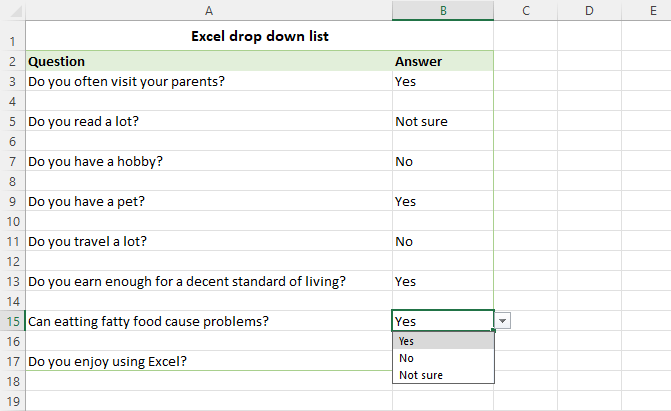
Excel drop down list, aka dropdown box or dropdown menu, is used to enter data in a spreadsheet from a predefined items list. When you select a cell containing the list, a small arrow appears next to the cell, so you click on it to make a selection.
The main purpose of using drop down lists in Excel is to limit the number of choices available for the user. Apart from that, a dropdown prevents spelling mistakes and makes data input faster and more consistent.
How to create drop down list in Excel
To make a drop-down list in Excel, use the Data Validation feature. Here are the steps:
- Select one or more cells where you want the picklist to appear. This can be a single cell, a range of cells, or a whole column. To select multiple non-contiguous cells, press and hold the Ctrl key.
- On the Data tab, in the Data Tools group, click Data Validation.
- On the Settings tab of the Data Validation dialog box, do the following:
- In the Allow box, select List.
- In the Source box, type the items separated by a comma with or without spaces. Or select a range of cells on the sheet containing the items.
- Make sure the In-cell dropdown box is checked (default), otherwise the drop-down arrow won't appear next to the cell.
- Select or clear the Ignore blank option depending on how you want to handle empty cells.
- When done, click OK.
Congratulations! You have successfully created a simple dropdown list in Excel. Now, your users can click an arrow next to a cell, and then select the entry they want.
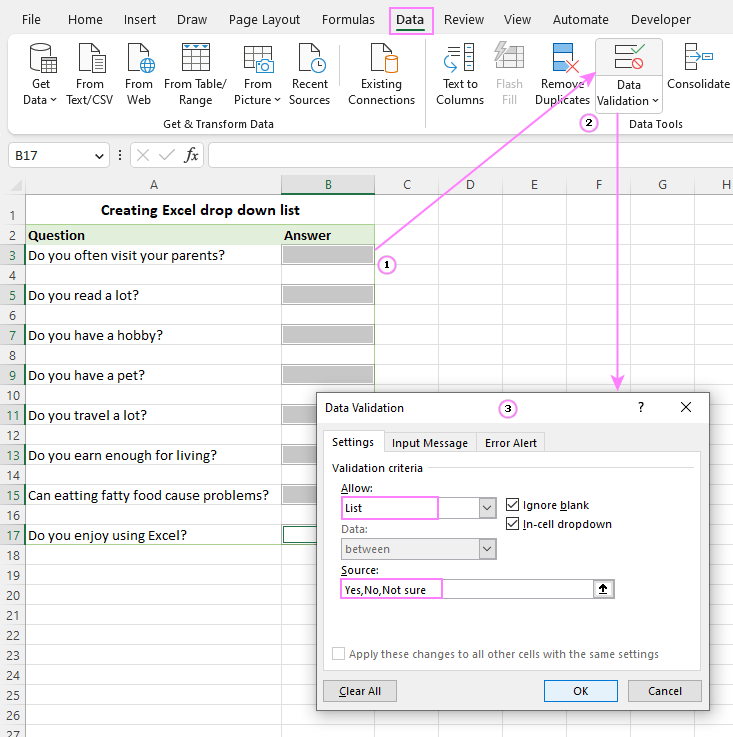
A drop down list of comma separated values works well for small data validation lists that are unlikely to ever change. For frequently updated lists, you'd better use a range or table for the source. The detailed step-by-step instructions for each method follow below.
Tip. To expedite data input in your Excel sheets, you can also use a data entry form.
Make drop-down menu from a range of cells
To insert a drop-down list based on the values input in a range of cells, carry out these steps:
- Start by creating a list of items that you want to include in the drop-down. For this, just type each item in a separate cell. This can be done in the same worksheet as the dropdown list or in a different sheet.
- Select the cell(s) that are to contain the list.
- On the ribbon, click the Data tab > Data Validation.
- In the Data Validation dialog window, select List from the Allow drop-down menu. Place the cursor in the Source box and select the range of cells containing the items, or click the Collapse Dialog icon and then select the range. When done, click OK.
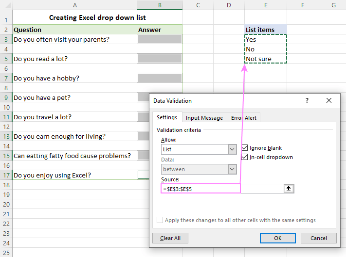
Advantages: You can modify your dropdown list by making changes in the referenced range without having to edit the data validation list itself.
Drawbacks: To add or remove items, you will need to update the Source range reference.
Insert drop down list from a named range
Initially, this method of creating an Excel data validation list takes a bit more time but may save even more time in the long run.
- Make a list of items on the sheet. The values should be entered into a single column or row without any blank cells.
Tip. It's a good idea to sort the items alphabetically or in a custom order you want them to appear in the drop-down menu.
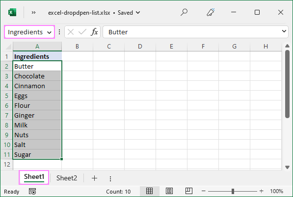
- Create a named range. The fastest way is to select the cells and type the desired name directly in the Name Box. When finished, click Enter to save the newly created named range. For more information, please see how to define a name in Excel.
As an example, let's create a range named Ingredients:
- Select the cells for the picklist - on the same sheet as the named range or in a different worksheet.
- Open the Data Validation dialog window and configure the rule:
- In the Allow box, select List.
- In the Source box, type an equals sign followed by the range name. In our case, it's =Ingredients.
- Click OK.
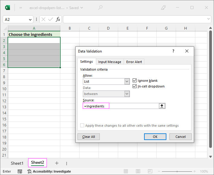
Note. If your named range has at least one blank cell, leaving the Ignore blank box selected allows typing any value in the validated cell.
Advantages: If you insert multiple drop-downs in different sheets, named ranges will make them a lot easier to identify and manage.
Drawbacks: Takes a bit more time to set up.
Create drop-down from Excel table
Instead of using a named range, you can place the source data into a fully functional Excel table. Why may you want to use a table? First and foremost, because it lets you create an expandable dynamic drop-down list that updates automatically as you add or remove items to/from the table.
To make a dynamic dropdown from an Excel table, follow these steps:
- Type the list items in a table or convert an existing range to a table using the Ctrl + T shortcut.
- Select the cell(s) where you wish to insert a dropdown.
- Open the Data Validation dialog window.
- Select List from the Allow drop-down box.
- In the Source box, enter the formula referring to a specific column in your table, not including the header cell. For this, use the INDIRECT function with a structured reference like this:
=INDIRECT("Table_name[Column_name]") - When done, click OK.
For this example, we're making a dropdown menu from the column named Ingredients in Table1:
=INDIRECT("Table1[Ingredients]")
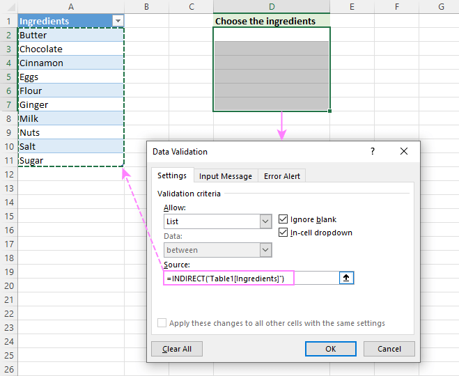
Advantages: Easy and quick way to insert an expandable dynamic drop down menu in Excel.
Drawbacks: Not found :)
How to create a dynamic dropdown list in Excel
If you regularly change the items in your picklist, the best approach is to create a dynamic drop down list. In this case, the list will update automatically in all the cells that contain whenever you add or remove items to/from the source list.
The fastest way to make a dynamic drop down in Excel is from a table as shown above. That is the default behavior of Excel tables; no extra settings or moves are required.
Another way is to use a regular named range and reference it with the OFFSET formula, as explained below.
- Type the items for the drop down menu in separate cells.
- Create a named formula. For this, press Ctrl + F3 to open the New Name dialog box. Type the name you want in the Name box, and then enter the following formula in the Refers to box.
=OFFSET(Sheet3!$A$2, 0, 0, COUNTA(Sheet3!$A:$A), 1)Where:
- Sheet3 - the sheet's name
- A - the column where the drop-down items are located
- $A$2 - the cell containing the first item
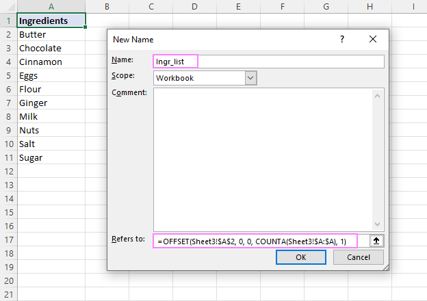
- With the formula name defined, create a dropdown based on a named range as usual.
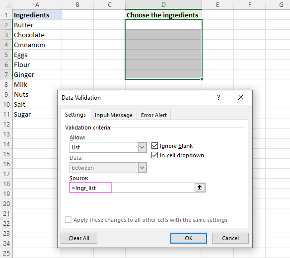
How this formula works
The formula comprises two functions - OFFSET and COUNTA. The COUNTA function counts all non-blanks in the specified column. OFFSET uses that count for the height argument, so it returns a reference to a range that includes only non-empty cells, starting from the cell containing the first item that you supply for the reference argument.
Advantages: The main advantage of a dynamic drop-down list is that you won't have to change the reference to the named range each time the source list is expanded or contracted. You simply delete or type new entries in the source list, and your dropdown menu will update automatically!
Drawbacks: A bit complex setup process.
Make a dynamic dropdown list in Excel 365/2021
Dynamic Array Excel has many innovative functions that are not available in older versions. One of these new functions named UNIQUE can help you create a dynamic drop-down with a simple formula.
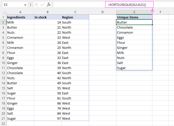
Suppose you have a dataset with many repeated items like in column A in the image below. You aim to add a dropdown list where each item appears just once.
To extract the unique items, use this formula:
=UNIQUE(A2:A21)
Optionally, you can sort the extracted values alphabetically by wrapping it in the SORT function:
=SORT(UNIQUE(A2:A21))
This dynamic array formula is entered just in one cell (E2) and it automatically spills into as many cells as needed to show all the unique items.
Next, you set up a drop down list using a spill range reference, which is a cell address followed by a hash character. In our case it's =$E$2# or =Sheet1!$E$2# if a dropdown is in another sheet:
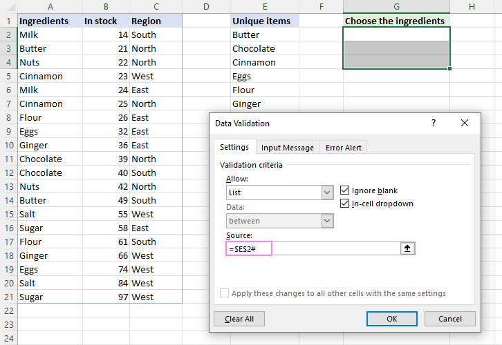
The result is an expandable dynamic drop-down list - the UNIQUE function automatically extracts new items as they are added to the source table, and the spill range reference forces Excel to update the drop-down list accordingly.
Tip. The same approach can be used to create a cascading drop-down list in Excel 365. For full details, please see Make a dynamic dependent dropdown list an easy way.
How to create drop down list from another sheet
To insert a drop-down menu that pulls data from a different worksheet, you can use a normal range, named range or Excel table:
- When making a dropdown menu from a named range, make sure the scope of the name is Workbook, and then set up a data validation list as usual.
- When creating a drop down list from a table, no extra steps are needed as table names/references are valid across the entire workbook.
- If you insert a drop down from a regular range, include the sheet's name in the source reference. In the Data Validation dialog window, place the cursor in the Source box, switch to the other sheet and select the range containing the items. Excel will add the sheet name to the reference automatically.
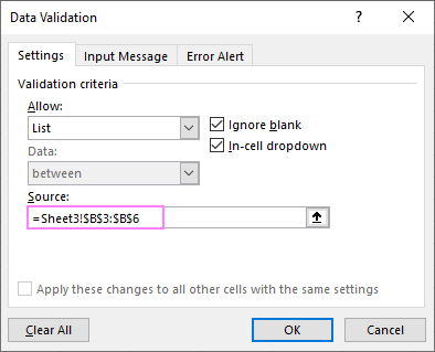
How to make drop-down list from another workbook
To create a drop-down menu in Excel using a list from another workbook as the source, you will have to define 2 named ranges - one in the source workbook and the other in the workbook where you wish to insert your Data Validation list. The steps are:
- In the source workbook, create a named range for the source list, say Source_list.
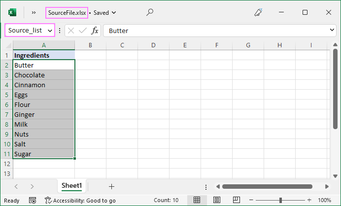
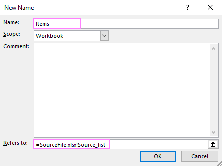
- In the main workbook, define a name that references your source list. For this example, we create the name Items that refers to:
=SourceFile.xlsx!Source_list
If the workbook's name contains spaces or non-alphabetical characters, it must be enclosed in single quotation marks like this:
='Source File.xlsx'!Source_list
For more details, please see How to make external reference in Excel.
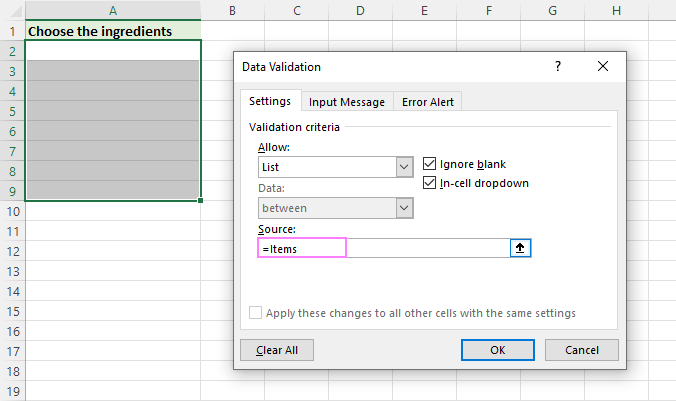
- In the main workbook, select the cell(s) for your picklist and click the Data tab > Data Validation. In the Source box, reference the name you created in step 2. In our case, it's =Items.
Notes:
- For the drop-down list from another workbook to work, the source workbook must be open.
- The dropdown list created in this way won't update automatically when items are added to or removed from the source list - you will have to modify the source list reference manually.
How to make a dynamic dropdown from another workbook
To create a dynamic dropdown list from another workbook, define a formula name in the source workbook using the OFFSET formula explained in Creating a dynamic drop-down in Excel. In this case, a dropdown menu in another workbook will be updated on the fly once any changes are made to the source list.
Searchable drop down list in Excel 365
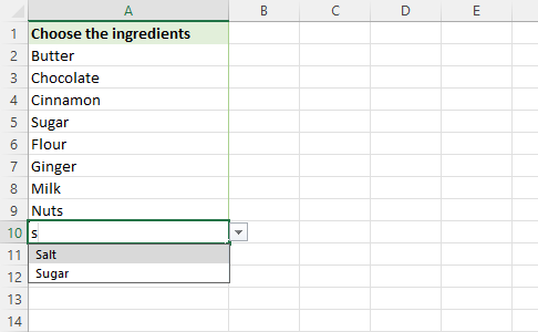
In Excel 365, data validation lists have an awesome AutoComplete feature. To speed up data entry in large lists, just start typing the target word in the dropdown menu cell - the autocomplete algorithm will match the typed substring with the dropdown list items and show you the found matches. As you type more characters, the displayed list is narrowed down, and conversely, when you remove characters, more matches are shown.
Insert a drop down list with message
To show an information message when someone clicks a dropdown list cell, proceed in this way:
- In the Data Validation dialog box, switch to the Input Message tab.
- Make sure the Show input message when cell is selected option is checked.
- Type the title and message in the corresponding fields (up to 225 characters).
- Click OK to save the message and close the dialog.
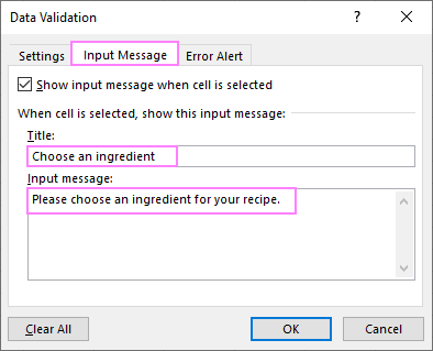
The resulting drop down list with message will look similar to this:
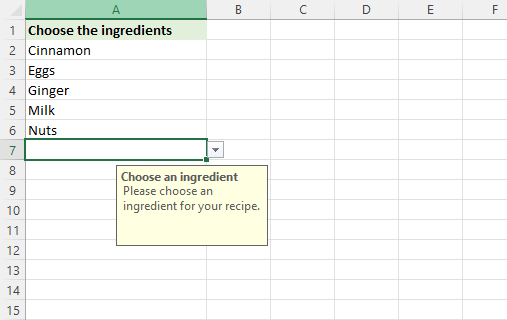
Make an editable drop down list in Excel
By default, an Excel drop-down is non-editable, i.e. restricted to the values in the list itself. If you type any other value, an error alert will show up. However, you can allow users to enter their own values. Here's how:
- Open the Data Validation dialog window.
- On the Error Alert tab, uncheck the Show error alert after invalid data is entered box.
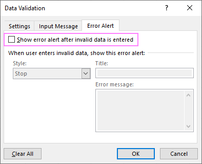
Technically, this turns a drop-down list into a combo box. The term "combo box" means an editable dropdown that allows users to either select a value from the predefined list or type a custom value directly in the box.
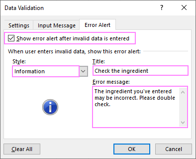
Optionally, you can display a warning message when someone attempts to enter a value that is not in the list:
- On the Error Alert tab, select the Show error alert after invalid data is entered option.
- From the Style box, pick either Information or Warning, and then type the title and message text.
- Information message is best to be used if there is nothing wrong with the user entering a custom value.
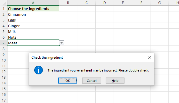
- Warning message will induce users to select an item from the drop-down box rather than enter their own data, though it does not prohibit it.
And here's an editable Excel dropdown list with a warning message in action:
Tip. If you are not sure what title or message text to type, you can leave the fields empty. In this case, Excel will display the default alert "This value does not match the data validation restrictions defined for this cell."
That's how to make a simple drop-down list in Excel. In the next article, we will explorer this topic further and learn how to insert a cascading (dependent) drop down list with conditional Data Validation. Please stay tuned and thank you for reading!
Practice workbook for download
Excel drop-down list - examples (.xlsx file)
 by
by
258 comments
First of all thanks for this detailed post - quite useful.
i have a point on the part where we create a drop down list using the OFFSET function
Because the COUNTA also counts the headers, the dropdown shows some blanks also at the end. This allows typing any value in the validated cell which may defeat the purpose of the validation itself.
To avoid this we can use one of the following workarounds -
1. Uncheck the Ignore blank box when creating the data validation, or
2. Reduce the header rows from COUNTA, for example if you have 1 header row in the column where you entered your range, use the following
=OFFSET(Sheet3!$A$2, 0, 0, COUNTA(Sheet3!$A:$A)-1, 1)
Hi I'm new to this and have picked up some great tips. I am struggling with a drop down menu, I can get the results of multiple choice, but results are displayed as a continuous line . How can i change this to show multiple lines the same as it is in the drop down?
Any assistance welcome thanks
Hi! If I understand your task correctly, try to use the recommendations described in this guide: How to create dropdown with multiple selections in separate lines. I hope my advice will help you solve your task.
Hi, is there any way to create 2 dropdown lists which are dependent on each other? I mean - second dropdown list has a different content depends on what will be chosen on the first one
Hi! You can find the examples and detailed instructions here: How to make a dependent (cascading) drop-down list in Excel and Create a dynamic dependent drop down list in Excel an easy way.
I have been trying to find a drop down in excel to provide examples for users and NOT data validation which restricts the data to exactly the same wording (not useful when you are trying to put things like a copyright and the user chooses the year, which can be any year, and different companies). Why is is so hard to find the answer?
Unfortunately, this information is not enough to understand what you need.
Hello! I've gotten further with your article than I have with others so I thank you for that. For the step Create drop-down from Excel table, I was able to do that and it worked as expected. However, I need to have more than one table. How do I add additional tables? Can you please provide what the formula would look like? This formula in data validation works perfectly for just one table....=INDIRECT("Table1[Grocery]") but again, need to add additional tables, if this is even possible. Thank you!!
Hi! You can only create a drop-down list from one data source. Therefore, you cannot use data from two tables for a drop-down list. You can merge the data from two tables using the VSTACK function and use a reference to that range of cells to create a drop-down list.
=VSTACK(INDIRECT("Table1[Ingredients]"),INDIRECT("Table2[Ingredients]"))
I hope my advice will help you solve your task.
hello
how should i filter the column ingredients
like blank
i can't find a solution for this
Hi! To filter values in Excel, you can use the Excel Filter tool. Read more: Excel Filter: How to add, use and remove. Using a formula, you can filter values using these guidelines: Excel FILTER function - dynamic filtering with formulas. If this is not what you need, clarify the question in more detail.
Hi, is it possible to have the source of a dropdown list be in 1 cell instead of a table. I have to restructure a sheet with tens to hundreds of dropdowns, if i put them all in different tables it becomes a mess. I'd like to make a table with all the sources of the dropdowns in 1 cell separated by a comma, in the same style as you'd input your data in the Data Validation window. Then i refer the source to this one cell instead of the table, I just don't know if it is even possible.
This would make my life much easier, thank you in advance
Edoe
Hi! Unfortunately, a drop down list with data from a single cell can only return a single value.
Okay, thank you
For some reason, this isn't working the way I need it to work. I want to be able to select an option from the drop down list, add some data and then repeat it for each option of the drop down list. For example: I want to click on Birmingham from the drop down list, add information about Birmingham and then when I click on the drop down and choose a different location like London, I want the sheet to be blank and add information to it. When everything is complete, I want to be able to click on the drop down list for each location to see that the data changes.
Hi! A drop-down list writes the selected value to a cell. But it cannot automatically change this value depending on some conditions. You can automatically remove values from cells when the value in a particular cell changes by using a VBA macro.
I'm struggling on how to do this because it's not working the way I need it too. I need to click on the drop down and for the information I type to change for each drop down. For example: I want to be able to click on Birmingham, I type in bits of data and then when I click on the drop down list to give me a different location like Bradford I want to be able to click on Bradford and type in new data. I want to be able to select different locations from the drop down list and for the information to change each time based on what I select from the drop down.
Like how did I not notice the searchable drop down list in excel. All these while I have been looking for a way to make my drop down list searchable but couldn’t. Thanks a lot😁
Google sent me to this article inaccurately.
I was looking on a way to exclude header from the dropdown while having directly inputted entries.
For example. I have this column named Medium with source entries as Email, Call, Text, Mail.
While it works, Excel puts a yellow error icon on the left side of "Medium' header. It says this entry "Header" is not part of the list.
I don't want to create the list separately on another cell or sheet.
Excel complicates it even more by adding a dropdown to table headers which chocks Excel.
I searched everywhere and could not find a solution
How to use vba to add drop-down menu?
I was not obliged to leave any comment but I had to simply write and to say this article is spot on and straight to the point. The author deserves a big thanks for making it look so easy. Ms. Svetlana Cheusheva thank you a million. From a user in Austria. Have a wonderful day!
Is it possible to create a drop down list where you can choose multiple entries? For example if one of the columns is food allergens, where you need to select multiple allergens from the drop down menu rather than just one.
Hi! If I understand your task correctly, this article may be helpful: How to make Excel drop down list with multiple selections.
Great content! I'm in a bit of a pickle. Looking for a solution. How can i create a searchable drop down list in excel but appending to the data as one selects from the value. Today, my excel runs a macro that would allow one to select multiple drop down values using a (;) to separate the selection within any given one cell. My users however, are looking for a searchable drop down, but with no interruptions to the current macro that would allow again for multiple drop down selections using the semicolon as the separator for each selection.
What can I use to satisfy this need?
Hi! In Excel 365, data validation lists have an AutoComplete feature. Read more about searchable drop down list in Excel 365 here. The macro for multi-select drop-down list does not work with Form Control and ActiveX Control elements.
How to I copy a dynamic drop down list from the source data page to the actual worksheet? It doesn't copy over
Hi! Maybe this article will be helpful: How to edit, copy and delete drop down list in Excel.
I've been using drop-down lists since the beginning of time, so I'm very familiar in setting this up and using it. Search in drop-down made my life so much easier, but recently it just stopped working - across all Excel sheets and workbooks that I open. I did not change anything - it is just not working - even if I use the mouse scroll button the scroll is not working, I have to drag down the little scroll bar in the box. I use Office 365, Windows Professional - I've done updates, restarted my laptop a thousand times, but no luck - does anyone know how I can fix this.
Hi! Specify how you searched in drop down list: with an ActiveX element or with a VBA macro in an ordinary drop down list. If the second option, there is probably a problem with the macro.
hi, pretty page but I do not found my problem...
I have a dropdown list with 26 entry BUT in use I can see always the first 8 and I have to srcoll down all the times if I wants to use an entry. My Question: can I prolong the presentation-list that I can see more of my list ???
many thanks and regards from germany
Hi!
To use more than 8 items to select values, you can use a combo box. For more information, read this instruction.
Hi, great site!
My question is if it is possible to edit the format of the drop-down box.
It is now 8 rows and i like it to have about 20?
Regrads,
Frans
Hi!
To use more than 8 rows to select values, you can use the combo box. See these instructions for details.
Hello Svetlana,
Congratulations on your articles and on what you or your loved ones are going through.
Concerning the paragraph Excel data validation list based on a table, I don't understand why you have to go through a named range. Can't we link directly to Table[[#data],[col_name]]? Maybe by coupling with an Indirect function?
Sincerely yours and congrat to all your team, the info you give is most valuable
Al1
Hello!
You are absolutely right - the combination of INDIRECT and table references works nicely. I've updated the instructions, thank you!
Hello,
It is a great article, I am from Pakistan when i am making a list like a1,a6,a12,a20 using this range hold the Control Button but this range not accepted in the list and giving a error I also used semi colon(;), but is also not accepted, it is only accepted continuous range like a1:a20 so please help
Very very helpful artical..
Thank you so much..
Have all success in your life.
VERY, VERY good & useful explanations. Thank you for taking the time to do this.
Hello Svetlana,
Thank you for a great tutorial and your through analysis and step by step presentation. You also did a wonderful job to explain the different options and pros and cons of each.
The only step that did not work for me was when I put the Table Name as the Data Source. The Database is in Sheet1, and the Table1 is in Sheet2 (column A, rows 2:30 with header on row 1).
Your input will be much appreciated. Thank you.
Joe
Hi Joe,
Thank you for your kind words about this article! You are right, the table method does not work in the current Excel version, though I can swear it did work back in 2014 when the tutorial was written.
Anyway, you can use the following workaround:
- After creating a table, create a named range for a column of data without including the heading cell. For example, you can define the name "Ingredients" that refers to =Table1[Ingredients].
- And then, create a data validation list based on the name.
This extra step may sound like a needless complication, but it does make your drop-down list expandable - when a new item is added to the table, it will appear in the list automatically.
I will update this part of the tutorial ASAP. Thank you for drawing my attention to this! :)
Hey Pretty..
I need your little help.. for Data validation can you help me...
hello svetlana. Is this article the Italian translation of your article?
https:// excelacademy.it/6623/creare-un-elenco-discesa-excel/
Hi Luke,
I do not speak Italian, but the contents seem very much alike :)
Another great article, thank you so much!
I've been using data validation based on table columns as my standard method since quite a while. However, there's one thing that annoys me: You have to create a separate named range for the table column (as you cannot put the table column reference as source into the data validation directly). Let's say I call the named range "Dropdown" and it refers to "Table[Column]" and has workbook scope.
Now, when I copy any sheet within the workbook a new instance of Dropdown is created automatically that has the new sheet as scope. I didn't find any way to avoid that. It even happens when I copy a sheet that does not use Dropdown at all.
Do you know how that can be avoided?
I have this problem to. A bug since I can delete those duplicate named ranges that have a worksheet scope and the validation list will still work since it's using the workbook scoped original named range.
Thank you very much sir, for the simplest explanation on how to edit items on the list. It made me reduce my stress for editing a form needed ASAP. Thank you very much.
Drop down list is not appearing on selection of arrow from begining.
Hi. Please have a look at the first "drop-down via comma-separated" option. You mention in step 3 to use a comma (,), however this should be a semi-colon (;).
Otherwise thanks for the great help.
Hello Jeanette!
The use of a semicolon or semicolon in formulas is determined by the regional settings of your Windows.
Great explanation. It solved my query in minutes. Thanks a lot!
Thank you for this very useful post! I was searching in the internet about providing a table as a source for the drop-down list. It solved my problem.
Dynamic drop down does not work, as prescribed.
I created a drop down list for expense type and created vlookup for tax rate based on expense type. However if user picks any expense type and then delete the entry then it gives an error message of NA in tax amount column. How can it be taken care of?
I have a query.
I have already populated some values in the drop down box.But now I want to insert a value in between the list of drop down values.
example,
I have suppose list of values 1,2,3,4....in my drop down list.
but now I want 1,2,6,7,3,4....(It means that I have to Insert two new values in between)how to do this? I have analysed all the ideas . Could anyone help in this?
Text size for drop down list is coming small. Is there a way to change the text size of the drop down list items.
I'm in the end. I didn't find solution to my problem with drop down menu.
The problem and question is, how to update already selected values from drop down menu, after that I changed original values in source table for drop down menu?
Because in Excel I have a list of hardware in many worplaces. And from time to time when workplace will change name I need to change it in Excel too.
And easiest way is to change/edit it in table for drop down menu, not to change it by add new workplace to table for drop down menu and then find hardware and select new work place from drop down menu. But now, when aj change some values in table for drop down menu, this change is not reflected in my list.
Just for sure: I'm not talking about adding new rows for drop down table.
Great lesson indeed! Thank you. Is there a way of choosing more than one item from the drop down menu. I do not understand VBS or anything that is outside Windows at all!
Good stuff!
Hi,
Awesome article!
However, when doing the dynamic one I copied the code in and changed the sheet name accordingly. However, it will only give me 88 rows and anything after this gets cut off.
Any idea what I am doing wrong?
Dear all,
I have a problem with defining the source of the drop down list.
When I click on another sheet for referencing the table where the list is, I can't. Excel just annoys me with an error sound and nothing shows. It doesn't go anywhere. I can't reference anything. What am I doing wrong? What should I do to overcome this. I'm using excel 2007.
thank you very much for your suport
I want to create a drop down in a table form.
eg. code budget actual variance percentage
Great job on this link. I was able to create a list on one workbook referencing another workbook and it worked perfectly. I now use the list to select parts and then populate other columns using VLOOKUP. Thanks for the article.
Hi,
You are very helpful!!!
I have a drop-down list with 8 items. When I open the drop-down, only 7 items appear and I have to scroll up to see the first item. Is there a way to always have the entire list show each time? I'm afraid my users will miss an option on the list.
Thanks.
Carl
Someone created a table for me but I need to add items to one of the lists which is located on a separate sheet. When I add the items to the list, they do not appear on the dropdown on my input sheet; only the original list appears. How do I add extra cells? I tried to do DataValidation but it does not add them. Thanks
Hi
I have a Worksheet_SelectionChange event procedure in a worksheet which make drop-down list automatically by selecting a specified cell in a column. But, after creation some drop-down list and selection of other cells for new drop-down list creation, I couldn't find the previous dro-down lists location.
Thanks