How to create external reference in Excel to refer to another sheet or workbook

Creating a reference to another sheet in Excel

When writing a formula that refers to cells in another worksheet, you can of course type that other sheet name followed by an exclamation point and a cell reference manually, but this would be a slow and error-prone way.

A better way is point to the cell(s) in another sheet that you want the formula to refer to, and let Excel take care of the correct syntax of your sheet reference. To have Excel insert a reference to another sheet in your formula, do the following:

1. Start typing a formula either in a destination cell or in the formula bar.
2. When it comes to adding a reference to another worksheet, switch to that sheet and select a cell or a range of cells you want to refer to.
3. Finish typing the formula and press the Enter key to complete it.

For example, if you have a list of sales figures in sheet Sales and you want to calculate the Value Added Tax (19%) for each product in another sheet named VAT, proceed in the following way:

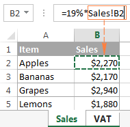
• Start typing the formula =19%* in cell B2 on sheet VAT.
• Switch to sheet Sales, and click on cell B2 there. Excel will immediately insert an external reference to that cell, as shown in the following screenshot:
  
• Press Enter to complete the formula.

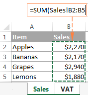
In a similar manner, you can reference a range of cells in another sheet. The only difference is that you select multiple cells on the source worksheet. For example, to find out the total of sales in cells B2:B5 on sheet Sales, you would enter the following formula:

=SUM(Sales!B2:B5)

This is how you reference another sheet in Excel. And now, let's see how you can refer to cells from a different workbook.

External reference to an open workbook

When the source workbook is open, an Excel external reference includes the workbook name in square brackets (including the file extension), followed by the sheet name, exclamation point (!), and the referenced cell or a range of cells. In other words, you use the following reference format for an open workbook reference:

For example, here's an external reference to cells B2:B5 on sheet Jan in the workbook named Sales.xlsx:

[Sales.xlsx]Jan!B2:B5

If you want, say, to calculate the sum of those cells, the formula with the workbook reference would look as follows:

=SUM([Sales.xlsx]Jan!B2:B5)

External reference to a closed workbook

When you reference another workbook in Excel, that other workbook does not necessarily need to be open. If the source workbook is closed, you must add the entire path to your external reference.

For example, to add up cells B2:B5 in the Jan sheet from Sales.xlsx workbook that resides within the Reports folder on drive D, you write the following formula:

=SUM(D:\Reports\[Sales.xlsx]Jan!B2:B5)

Here's a breakdown of the reference parts:

• File Path. It points to the drive and directory in which your Excel file is stored (D:\Reports\ in this example).
• Workbook Name. It includes the file extension (.xlsx, .xls, or .xslm) and is always enclosed in square brackets, like [Sales.xlsx] in the above formula.
• Sheet Name. This part of the Excel external reference includes the sheet name followed by an exclamation point where the referenced cell(s) is located (Jan! in this example).
• Cell Reference. It points to the actual cell or a range of cells referenced in your formula.

If you've created an reference to another workbook when that workbook was open, and after that you closed the source workbook, your external workbook reference will get updated automatically to include the entire path.

Making a reference to another workbook in Excel

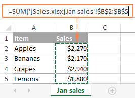
As is the case with creating an Excel formula that references another sheet, you don't have to type a reference to a different workbook manually. Just switch to the other workbook when entering your formula, and select a cell or a range of cells you want to refer to. Microsoft Excel will take care of the rest:

Creating a name in Excel

To create a name in Excel, select all the cells you want to include, and then either go to the Formulas tab > Defined names group and click the Define name button, or press Ctrl + F3 and click New.

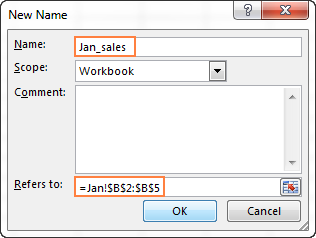
In the New Name dialog, type any name you want (remember that spaces are not allowed in Excel names), and check if the correct range is displayed in the Refers to field.

For example, this is how we create a name (Jan_sales) for cells B2:B5 in Jan sheet:

Once the name is created, you are free to use it in your external references in Excel. The format of such references is much simpler than the format of an Excel sheet reference and workbook reference discussed earlier, which makes the formulas with name references easier to comprehend.

It's recommended that you always create workbook-level names (unless you have a specific reason not to), because they significantly simplify creating Excel external references, as illustrated in the following examples.

Referencing a name in another sheet in the same workbook

To reference a global workbook-level name in the same workbook, you simply type that name in a function's argument:

For example, to find the sum of all the cells within the Jan_sales name that we created a moment ago, use the following formula:

=SUM(Jan_sales)

To reference a local worksheet-level name in another sheet within the same workbook, you need to precede the name with the sheet name followed by an exclamation mark:

=Function(Sheet_name!name)

For example:

=SUM(Jan!Jan_sales)

If the sheet names includes spaces or mon-alphabetic chars, remember to enclose it in single quotes, e.g.:

=SUM('Jan report'!Jan_Sales)

Referencing a name in another workbook

A reference to a workbook-level name in a different workbook consists of the workbook name (including the extension) followed by an exclamation point, and the defined name (named range):

For example:

=SUM(Sales.xlsx!Jan_sales)

To reference a worksheet-level name in another workbook, the sheet name followed by the exclamation point should be included as well, and the workbook name should be enclosed in square brackets. For example:

=SUM([Sales.xlsx]Jan!Jan_sales)

When referencing a named range in a closed workbook, remember to include the full path to your Excel file, for example:

=SUM('C:\Documents\Sales.xlsx'!Jan_sales)

How to create an Excel name reference

If you have created a handful of different names in your Excel sheets, you don't need to remember all those names by heart. To insert an Excel name reference in a formula, perform the following steps:

1. Select the destination cell, enter the equal sign (=) and start typing your formula or calculation.
2. When it comes to the part where you need to insert an Excel name reference, do one of the following:
   • If you are referring to a workbook-level name from another workbook, switch to that workbook. If the name resides in another sheet within the same workbook, skip this step.
   • If you are making a reference to a worksheet-level name, navigate to that specific sheet either in the current or different workbook.
3. Press F3 to open the Past Name dialog window, select the name you want to refer to, and click OK.
   
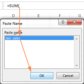
4. Finish typing your formula or calculation and press the Enter key.