The tutorial shows how to make custom Data Validation rules in Excel. You will find a few examples of Excel data validation formulas to allow only numbers or text values in specific cells, or only text beginning with specific characters, permit unique data preventing duplicates, and more.
In yesterday's tutorial we started to look at Excel Data Validation - what its purpose is, how it works, and how to use built-in rules to validate data in your worksheets. Today, we are going to take a step further and talk about the nitty-gritty aspects of custom data validation in Excel as well as experiment with a handful of different validation formulas.
How to create custom data validation with formula
Microsoft Excel has several built-in data validation rules for numbers, dates and text, but they cover only the most basic scenarios. If you want to validate cells with your own criteria, create a custom validation rule based on a formula. Here's how:
- Select one or more cells to validate.
- Open the Data Validation dialog box. For this, click the Data Validation button on the Data tab, in the Data Tools group or press the key sequence Alt > D > L (each key is to be pressed separately).
- On the Settings tab of the Data Validation dialog window, select Custom in the Allow box, and enter your data validation formula in the Formula box.
- Click OK.
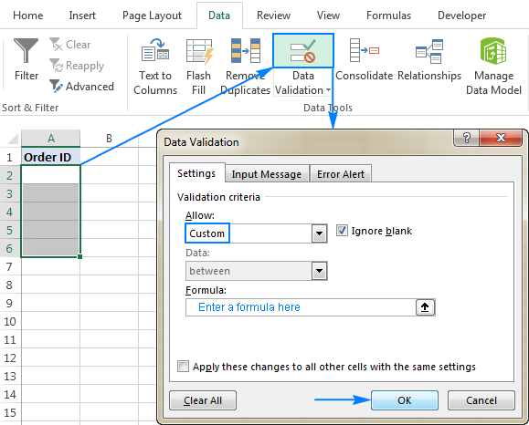
Optionally, you can add a custom input message and Error alert that will show up when the user selects the validated cell or enters invalid data, respectively.
Below you will find a few examples of custom validation rules for different data types.
Note. All Excel data validation rules, built-in and custom, verify only new data that is typed in a cell after creating the rule. Copied data is not validated, nor is the data input in the cell before making the rule. To pin down existing entries that do not meet your data validation criteria, use the Circle Invalid Data feature as shown in How to find invalid data in Excel.
Excel data validation to allow numbers only
Surprisingly, none of the inbuilt Excel data validation rules cater for a very typical situation when you need to restrict users to entering only numbers in specific cells. But this can be easily done with a custom data validation formula based on the ISNUMBER function, like this one:
=ISNUMBER(C2)
Where C2 is the topmost cell of the range you want to validate.
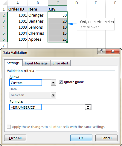
Note. The ISNUMBER function allows any numeric values in validated cells, including integers, decimals, fractions as well as dates and times, which are also numbers in terms of Excel.
Excel data validation to allow text only
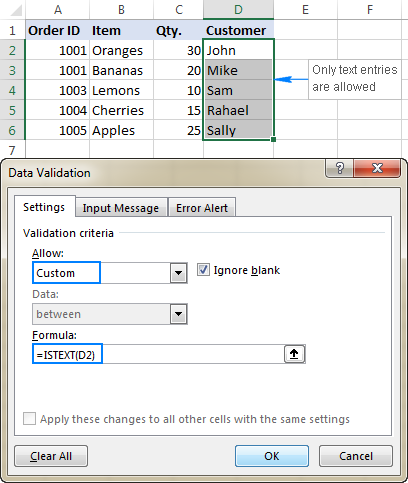
If you are looking for the opposite - to allow only text entries in given range of cells, then build a custom rule with the ISTEXT function, for example:
=ISTEXT(D2)
Where D2 is the uppermost cell of the selected range.
Allow text beginning with specific character(s)
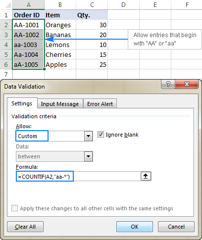
If all values in a certain range should begin with a particular character or substring, then do Excel data validation based on the COUNTIF function with a wildcard character:
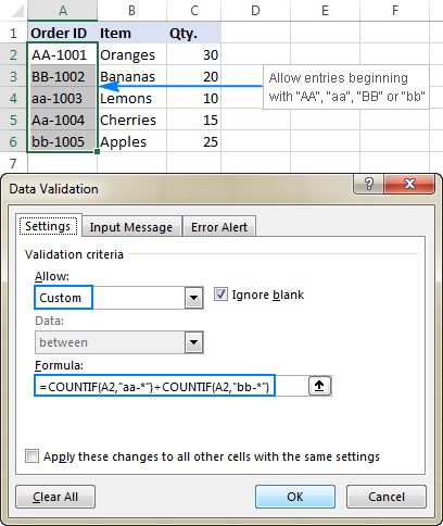
For example, to ensure that all order id's in column A begin with the "AA-", "aa-", "Aa-", or "aA-" prefix (case-insensitive), define a custom rule with this data validation formula:
=COUNTIF(A2,"aa-*")
Validation formula with the OR logic (multiple criteria)
In case there are 2 or more valid prefixes, add up several COUNTIF functions, so that your Excel data validation rule works with the OR logic:
=COUNTIF(A2,"aa-*")+COUNTIF(A2,"bb-*")
Case-sensitive validation formula
If the character case matters, then use EXACT in combination with the LEFT function to create a case-sensitive validation formula for entries beginning with specific text:
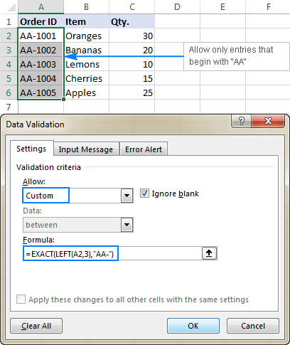
For instance, to allow only those order ids that begin with "AA-" (neither "aa-" nor "Aa-" is allowed), use this formula:
=EXACT(LEFT(A2,3),"AA-")
In the above formula, the LEFT function extracts the first 3 characters from cell A2, and EXACT performs a case-sensitive comparison with the hard-coded substring ("AA-" in this example). If the two substrings match exactly, the formula returns TRUE and the validation passes; otherwise FALSE is returned and the validation fails.
Allow entries containing certain text
To allow entries that contain specific text anywhere in a cell (in the beginning, middle, or end), use the ISNUMBER function in combination with either FIND or SEARCH depending on whether you want case-sensitive or case-insensitive match:
- Case-insensitive validation:
ISNUMBER(SEARCH(text, cell))
- Case-sensitive validation:
ISNUMBER(FIND(text, cell))
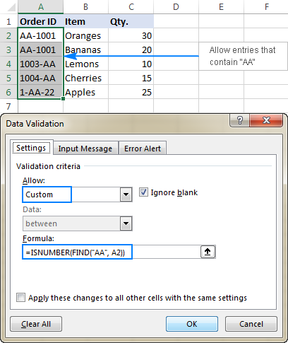
On our sample data set, to permit only entries containing the text "AA" in cells A2:A6, use one of these formulas:
Case-insensitive:
=ISNUMBER(SEARCH("AA", A2))
Case-sensitive:
=ISNUMBER(FIND("AA", A2))
The formulas work with the following logic:
You search the substring "AA" in cell A2 using FIND or SEARCH, and both return a position of the first character in the substring. If the text is not found, an error is returned. For any numeric value returned as the result of search, the ISNUMBER function yields TRUE, and data validation is successful. In case of an error, ISNUMBER returns FALSE, and the entry won't be allowed in a cell.
Data validation to allow only unique entries and disallow duplicates
In situations when a certain column or a range of cell should not contain any duplicates, configure a custom data validation rule to allow only unique entries. For this, we are going to use the classic COUNTIF formula to identify duplicates:
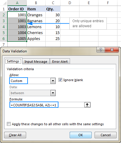
For example, to make sure that only unique order ids are input in cells A2 to A6, create a custom rule with this data validation formula:
=COUNTIF($A$2:$A$6, A2)<=1
When a unique value is entered, the formula returns TRUE and the validation succeeds. If the same value already exists in the specified range (count greater than 1), COUNTIF returns FALSE and the input fails validation.
Please pay attention that we lock the range with absolute cell references (A$2:$A$6) and use a relative reference for the top cell (A2) to get the formula to adjust properly for each cell in the validated range.
Note. This data validation formulas is case-insensitive, it does not distinguish uppercase and lowercase text.
Validation formulas for dates and times
Inbuilt date validation provides quite a lot of predefined criteria to restrict users to entering only dates between the two dates you specify, greater than, less than, or equal to a given date.
If you want more control over data validation in your worksheets, you can replicate the inbuilt functionality with a custom rule or write your own formula that goes beyond the built-in capabilities of Excel data validation.
Allow dates between two dates
To limit the entry to a date within a specified range, you can use either the predefined Date rule with the "between" criteria or make a custom validation rule with this generic formula:
Where:
- cell is the topmost cell in the validated range, and
- start and end dates are valid dates supplied via the DATE function or references to cells containing the dates.
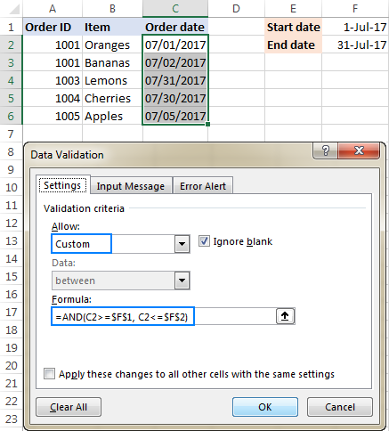
For example, to allow only dates in the month of July of the year 2017, use the following formula:
=AND(C2>=DATE(2017,7,1),C2<=DATE(2017,7,31))
Or, enter the start date and end date in some cells (F1 and F2 in this example), and reference those cells in your formula:
=AND(C2>=$F$1, C2<=$F$2)
Please notice that the boundary dates are locked with absolute cell references.
Allow weekdays or weekends only
To restrict a user to entering only weekdays or weekends, configure a custom validation rule based on the WEEKDAY function.
With the return_type argument set to 2, WEEKDAY returns an integer ranging from 1 (Monday) to 7 (Sunday). So, for weekdays (Mon to Fri) the result of the formula should be less than 6, and for weekends (Sat and Sun) greater than 5.
Allow only workdays:
Allow only weekends:
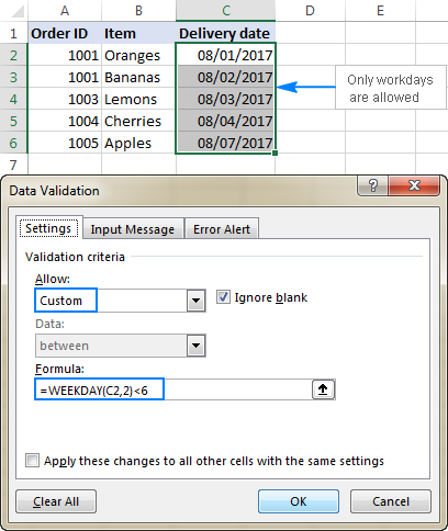
For example, to allow entering only workdays in cells C2:C6, use this formula:
=WEEKDAY(C2,2)<6
Validate dates based on today's date
In many situations, you may want to use today's date as the start date of the allowed date range. To get the current date, use the TODAY function, and then add the desired number of days to it to compute the end date.
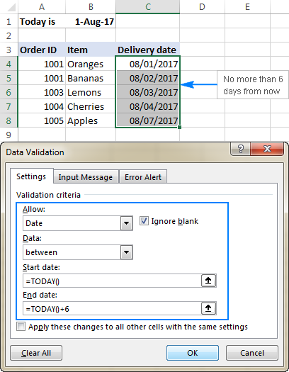
For example, to limit the data entry to 6 days from now (7 days including today), we are going to use the built-in Date rule with the formula-based criteria:
- Select Date in the Allow
- Select between in the Data
- In the Start date box, enter
=TODAY() - In the End date box, enter
=TODAY() + 6
In a similar manner, you can restrict users to entering dates before or after today's date. For this, select either less than or greater than in the Data box, and then enter =TODAY() in the End date or Start date box, respectively.
Validate times based on current time
To validate data based on the current time, use the predefined Time rule with your own data validation formula:
- In the Allow box, select Time.
- In the Data box, pick either less than to allow only times before the current time, or greater than to allow times after the current time.
- In the End time or Start time box (depending on which criteria you selected on the previous step), enter one of the following formulas:
- To validate dates and times based on the current date and time:
=NOW() - To validate times based on the current time:
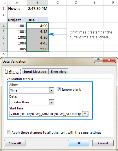
=TIME( HOUR(NOW()), MINUTE(NOW()), SECOND(NOW()))
- To validate dates and times based on the current date and time:
The screenshot below shows a rule that allows only times greater than the current time:
Custom Excel data validation rule not working
If your formula-based data validation rule does not work as expected, there are 3 main points to check:
- Data validation formula is correct
- Validation formula does not refer to an empty cell
- Appropriate cell references are used
Check the correctness of your Excel data validation formula
For starters, copy your validation formula into some cell to make sure it does not return an error such as #N/A, #VALUE or #DIV/0!.
If you are creating a custom rule, the formula should return the logical values of TRUE and FALSE or the values of 1 and 0 equating to them, respectively.
If you use a formula-based criteria in a built-in rule (like we did to validate times based on the current time), it can also return another numeric value.
Excel data validation formula should not refer to an empty cell
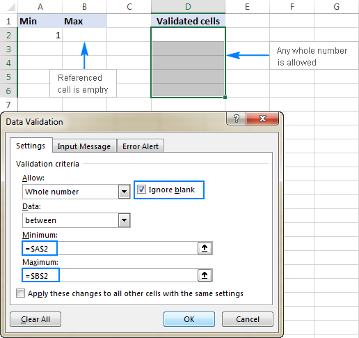
In many situations, if you select the Ignore blank box when defining the rule (usually selected by default) and one or more cells referenced in your formula is blank, any value will be allowed in the validated cell.
Here is an example in the simplest form:
Absolute and relative cell references in data validation formulas
When setting up a formula-based Excel validation rule, please keep in mind that all cell references in your formula are relative to the upper left cell in the selected range.
If you are creating a rule for more than one cell and your validation criteria are dependent on specific cells, be sure to use absolute cell references (with the $ sign like $A$1), otherwise your rule will work correctly only for the first cell. To better illustrate the point, please consider the following example.
Supposing, you want to restrict data entry in cells D2 to D5 to whole numbers between 1 (minimum value) and the result of dividing A2 by B2. So, you calculate the maximum value with this simple formula =A2/B2, like shown in the screenshot below:
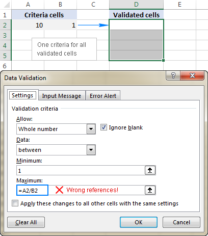
The problem is this seemingly correct formula won't work for cells D3 to D5 because relative references change based on a relative position of rows and columns. Thus, for cell D3 the formula will change to =A3/B3, and for D4 it will become =A4/B4, doing data validation all wrong!
To fix the formula, just type "$" before the column and row references to lock them: =$A$2/$B$2. Or, press F4 to toggle between different reference types.
In situations when you want to validate each cell based on its own criteria, use relative cell references without $ sign to get the formula to adjust for each row or/and column:
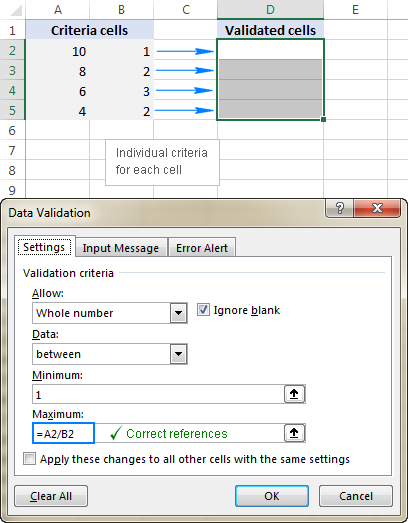
As you see, there is no "absolute truth", the same formula could be right or wrong depending on situation and your particular task.
This is how to use data validation in Excel with your own formulas. T gain more understanding, feel free to download our sample workbook below and examine the rule settings. I thank you for reading and hope to see you on our blog next week!
Practice workbook for download
Excel Data Validation examples (.xlsx file)
 by
by
274 comments
Hello,
I am trying to come up with a formula to only allow a 9 digit number, or a 9 digit number with an R or G at the end. We have certin profile numbers we use at my place of work and want to make sure no one mistypes anything. For example, the entries could be 123451234 or 123121234G or 123121234R with no spaces, dashes, etc.
Hello!
We have a special tutorial that can help to solve your problem. You can find the examples and detailed instructions here: Excel Data Validation using regular expressions.
Try using this formula to data validation:
=OR(RegExpMatch(A1,"^\d{9}[RG]"), RegExpMatch(A1,"^\d{9}"))
I hope that the advice I have given you will help you solve your problem.