The tutorial looks at how to get unique values in Excel by using the UNIQUE function and dynamic arrays. You will learn a simple formula to find unique values in a column or row, in multiple columns, based on conditions, and a lot more.
In the previous versions of Excel, extracting a list of unique values was a hard challenge. We have a special article that shows how to find uniques that occur just once, extract all distinct items in a list, ignore blanks, and more. Each task required a combined use of several functions and a multi-line array formula that only Excel gurus can fully understand.
The introduction of the UNIQUE function in Excel 365 has changed everything! What used to be a rocket science becomes as easy as ABC. Now, you don't need to be a formula expert to get unique values from a range, based on one or multiple criteria, and arrange the results in alphabetical order. All is done with simple formulas that everyone can read and adjust for your own needs.
Excel UNIQUE function
The UNIQUE function in Excel returns a list of unique values from a range or array. It works with any data type: text, numbers, dates, times, etc.
The function is categorized under Dynamic Arrays functions. The result is a dynamic array that automatically spills into the neighboring cells vertically or horizontally.
The syntax of the Excel UNIQUE function is as follows:
Where:
Array (required) - the range or array from which to return unique values.
By_col (optional) - a logical value indicating how to compare data:
- TRUE - compares data across columns.
- FALSE or omitted (default) - compares data across rows.
Exactly_once (optional) - a logical value that defines what values are considered unique:
- TRUE - returns values that occur only once, which is the database notion of unique.
- FALSE or omitted (default) - returns all distinct (different) values in the range or array.
Note. Currently the UNIQUE function is only available in Excel for Microsoft 365 and Excel 2021. Excel 2019, 2016 and earlier do not support dynamic array formulas, so the UNIQUE function is not available in these versions.
Basic UNIQUE formula in Excel
Below is an Excel unique values formula in its simplest form.
The goal is to extract a list of unique names from the range B2:B10. For this, we enter the following formula in D2:
=UNIQUE(B2:B10)
Please notice that the 2nd and 3rd arguments are omitted because the defaults work perfectly in our case - we are comparing the rows against each other and wish to return all the different names in the range.
When you press the Enter key to complete the formula, Excel will output the first found name in D2 spilling the other names into the cells below. As the result, you have all the unique values in a column:
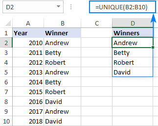
In case your data is across the columns from B2 to I2, set the 2nd argument to TRUE to compare the columns against each other:
=UNIQUE(B2:I2,TRUE)
Type the above formula in B4, press Enter, and the results will spill horizontally into the cells to the right. Thus, you'll get the unique values in a row:

Tip. To find unique values in a multi-column arrays and return them in one column or row, use UNIQUE together with the TOCOL or TOROW function as shown in the below examples:
Excel UNIQUE function - tips and notes
UNIQUE is a new function and like other dynamic array functions has a few specificities that you should be aware of:
- If the array returned by UNIQUE is the final result (i.e. not passed to another function), Excel dynamically creates an appropriately sized range and populates it with the results. The formula needs to be entered only in one cell. It is important that you have enough empty cells down and/or to the right of the cell where you enter the formula, otherwise a #SPILL error occurs.
- The results update automatically when the source data changes. However, new entries that are added outside of the referenced array are not included in the formula unless you change the array reference. If you want the array to respond to the resizing of the source range automatically, then convert the range to an Excel table and use structured references, or create a dynamic named range.
- Dynamic arrays between different Excel files only work when both workbooks are open. If the source workbook is closed, a linked UNIQUE formula will return a #REF! error.
- Like other dynamic array functions, UNIQUE can only be used within a normal range, not a table. When put within Excel tables, it returns a #SPILL! error.
How to find unique values in Excel - formula examples
The below examples show some practical uses of the UNIQUE function in Excel. The main idea is to extract unique values or remove duplicates, depending on your viewpoint, in the simplest possible way.
Extract unique values that occur only once
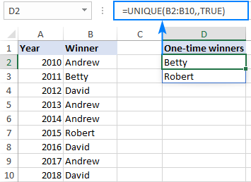
To get a list of values that appear in the specified range exactly once, set the 3rd argument of UNIQUE to TRUE.
For example, to pull the names that are on the winners list one time, use this formula:
=UNIQUE(B2:B10,,TRUE)
Where B2:B10 is the source range and the 2nd argument (by_col) is FALSE or omitted because our data is organized in rows.
Find distinct values that occur more than once
If you are pursuing an opposite goal, i.e. are looking to get a list of values that appear in a given range more than one time, then use the UNIQUE function together with FILTER and COUNTIF:
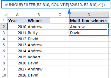
For example, to extract different names that occur in B2:B10 more than once, you can use this formula:
=UNIQUE(FILTER(B2:B10, COUNTIF(B2:B10, B2:B10)>1))
How this formula works:
At the heart of the formula, the FILTER function filters out duplicate entries based on the count of occurrences, returned by the COUNTIF function. In our case, the result of COUNTIF is this array of counts:
{4;1;3;4;4;1;3;4;3}
The comparison operation (>1) changes the above array to TRUE and FALSE values, where TRUE represents the items that appear more than once:
{TRUE;FALSE;TRUE;TRUE;TRUE;FALSE;TRUE;TRUE;TRUE}
This array is handed off to FILTER as the include argument, telling the function which values to include in the resulting array:
{"Andrew";"David";"Andrew";"Andrew";"David";"Andrew";"David"}
As you can notice, only the values corresponding to TRUE survive.
The above array goes to the array argument of UNIQUE, and after removing duplicates it outputs the final result:
{"Andrew";"David"}
Tip. In a similar fashion, you can filter unique values that occur more than twice (>2), more than three times (>3), etc. For this, simply change the number in the logical comparison.
Find unique values in multiple columns (unique rows)
In situation when you want to compare two or more columns and return the unique values between them, include all the target columns in the array argument.
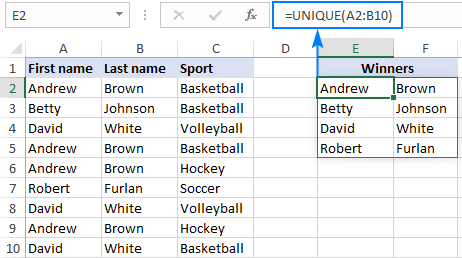
For instance, to return the unique First name (column A) and Last name (column B) of the winners, we enter this formula in E2:
=UNIQUE(A2:B10)
Pressing the Enter key yields the following results:
To get unique rows, i.e. the entries with the unique combination of values in columns A, B and C, this is the formula to use:
=UNIQUE(A2:C10)
Amazingly simple, isn't it? :)
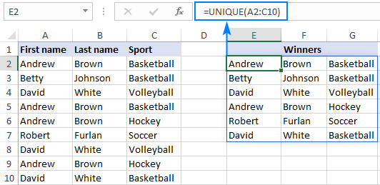
Get a list of unique values sorted in alphabetical order
How do you usually alphabetize in Excel? Right, by using the inbuilt Sort or Filter feature. The problem is you need to re-sort every time your source data changes, because unlike Excel formulas that recalculate automatically with every change in the worksheet, the features have to be re-applied manually.
With the introduction of dynamic array functions this problem is gone! What you need to do is simply warp the SORT function around a regular UNIQUE formula, like this:
For example, to extract unique values in columns A through C and arrange the results from A to Z, use this formula:
=SORT(UNIQUE(A2:C10))
Compared to the above example, the output is a lot easier to perceive and work with. For instance, we can clearly see that Andrew and David have been winners in two different sports.
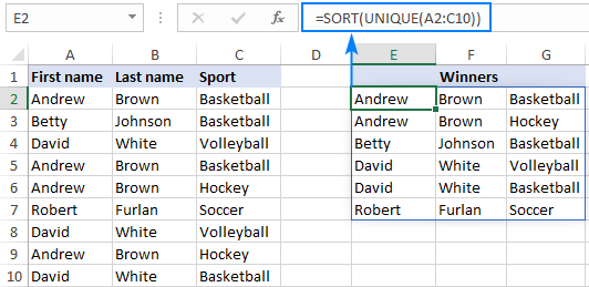
Tip. In this example, we sorted the values in the 1st column from A to Z. These are the defaults of the SORT function, therefore the optional sort_index and sort_order arguments are omitted. If you want to sort the results by some other column or in a different order (from Z to A or from highest to smallest) set the 2nd and 3rd arguments as explained in the SORT function tutorial.
Find unique values in multiple columns and concatenate into one cell
When searching in multiple columns, by default, the Excel UNIQUE function outputs each value in a separate cell. Perhaps, you'll find it more convenient to have the results in a single cell?
To achieve this, instead of referencing the entire range, use the ampersand (&) to concatenate the columns and put the desired delimiter in between.
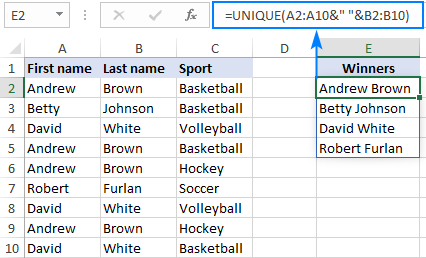
As an example, we are concatenating the first names in A2:A10 and the last names in B2:B10, separating the values with a space character (" "):
=UNIQUE(A2:A10&" "&B2:B10)
As the result, we have a list of full names in one column:
Get a list of unique values based on criteria
To extract unique values with condition, use the Excel UNIQUE and FILTER functions together:
- The FILTER function limits the data only to values that meet the condition.
- The UNIQUE function removes duplicates from the filtered list.
Here's the generic version of the filtered unique values formula:
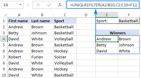
For this example, let's get a list of winners in a specific sport. For starters, we input the sport of interest in some cell, say F1. And then, use the below formula to get the unique names:
=UNIQUE(FILTER(A2:B10, C2:C10=F1))
Where A2:B10 is a range to search for unique values and C2:C10 is the range to check for the criteria.
Filter unique values based on multiple criteria
To filter unique values with two or more conditions, use the expressions like shown below to construct the required criteria for the FILTER function:
The result of the formula is a list of unique entries for which all of the specified conditions are TRUE. In terms of Excel, this is called the AND logic.
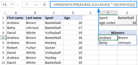
To see the formula in action, let's get a list of unique winners for the sport in G1 (criteria 1) and under the age in G2 (criteria 2).
With the source range in A2:B10, sports in C2:C10 (criteria_range 1) and ages in D2:D10 (criteria_range 2), the formula takes this form:
=UNIQUE(FILTER(A2:B10, (C2:C10=G1) * (D2:D10<G2)))
And returns exactly the results we are looking for:
How this formula works:
Here's a high-level explanation of the formula's logic:
In the include argument of the FILTER function, you supply two or more range/criteria pairs. The result of each logical expression is an array of TRUE and FALSE values. The multiplication of the arrays coerces the logical values to numbers and produces an array of 1's and 0's. Since multiplying by zero always gives zero, only the entries that meet all the conditions have 1 in the final array. The FILTER function filters out the items corresponding to 0 and hands off the results to UNIQUE.
For more information, please see FILTER with multiple criteria using AND logic.
Filter unique values with multiple OR criteria
To get a list of unique values based on multiple OR criteria, i.e. when this OR that criterion is TRUE, add the logical expressions instead of multiplying them:
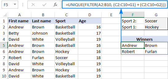
For example, to show the winners in either Soccer or Hockey, you can use this formula:
=UNIQUE(FILTER(A2:B10, (C2:C10="Soccer") + (C2:C10="Hockey")))
If needed, you can of course enter the criteria in separate cells and refer to those cells like shown below:
=UNIQUE(FILTER(A2:B10, (C2:C10=G1) + (C2:C10=G2)))
How this formula works:
Just like when testing multiple AND criteria, you place several logical expressions in the include argument of the FILTER function, each of which returns an array of TRUE and FALSE values. When these arrays are added up, the items for which one or more criteria is TRUE will have 1, and the items for which all the criteria are FALSE will have 0. As the result, any entry that meets any single condition makes it into the array that is handed over to UNIQUE.
For more information, please see FILTER with multiple criteria using OR logic.
Get unique values in Excel ignoring blanks
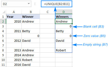
If you are working with a data set that contains some gaps, a list of uniques obtained with a regular formula is likely to have an empty cell and/or zero value. This happens because the Excel UNIQUE function is designed to return all distinct values in a range, including blanks. So, if your source range has both zeros and blank cells, the unique list will contain 2 zeros, one representing a blank cell and the other - a zero value itself. Additionally, if the source data contains empty strings returned by some formula, the uique list will also include an empty string ("") that visually looks like a blank cell:
To get a list of unique values without blanks, this is what you need to do:
- Filter out blank cells and empty strings by using the FILTER function.
- Utilize the UNIQUE function to limit results to unique values only.
In a generic form, the formula looks as follows:
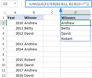
In this example, the formula in D2 is:
=UNIQUE(FILTER(B2:B12, B2:B12<>""))
As the result, Excel returns a list of unique names without empty cells:
Note. In case the original data contains zeros, one zero value will be included in the unique list.
Find unique values in specific columns
Sometimes you may want to extract unique values from two or more columns that are not adjacent to each other. At times, you may also want to re-order the columns in the resulting list. Both tasks can be fulfilled with help of CHOOSE function.
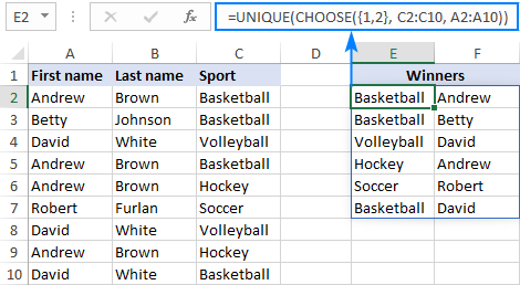
From our sample table, suppose you wish to get a list of winners based on the values in columns A and C and arrange the results in this order: first a sport (column C), and then a sportsman name (column A). To have it done, we construct this formula:
=UNIQUE(CHOOSE({1,2}, C2:C10, A2:A10))
And get the following result:
How this formula works:
The CHOOSE function returns a 2-dimentional array of values from the specified columns. In our case, it also swaps the order of columns.
{"Basketball","Andrew"; "Basketball","Betty"; "Volleyball","David"; "Basketball","Andrew"; "Hockey","Andrew"; "Soccer","Robert"; "Volleyball","David"; "Hockey","Andrew"; "Basketball","David"}
From the above array, the UNIQUE function returns a list of unique records.
Find unique values and handle errors
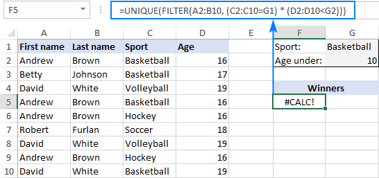
The UNIQUE formulas we've discussed in this tutorial work just perfect… provided there is at least one value that meets the specified criteria. If the formula does not find anything, a #CALC! error occurs:
To prevent this from happening, simply wrap your formula in the IFERROR function.
For example, if no unique values meeting the criteria are found, you can display nothing, i.e. an empty string (""):
=IFERROR(UNIQUE(FILTER(A2:B10, (C2:C10=G1) * (D2:D10<G2))), "")
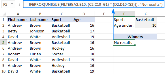
Or you can clearly inform your users that no results are found:
=IFERROR(UNIQUE(FILTER(A2:B10, (C2:C10=G1) * (D2:D10<G2))), "No results")
Excel UNIQUE function not working
As you have seen, the emergence of the UNIQUE function has made finding unique values in Excel incredibly easy. If all of a sudden your formula results in an error, it's most likely to be one of the following.
#NAME? error
Occurs if you use a UNIQUE formula in an Excel version where this function is not supported.
Currently, the UNIQUE function is only available in Excel 365 and 2021. If you have a different version, you may find an appropriate solution in this tutorial: How to get unique values in Excel 2019, Excel 2016 and earlier.
The #NAME? error in supported versions indicates that the function's name is misspelled. For more details, see How to fix #NAME error in Excel.
#SPILL error
Occurs if one or more cells in the spill range are not completely blank.
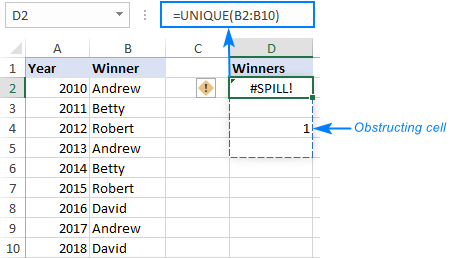
To fix the error, just clear or delete non-empty cells. To see exactly which cells are getting in the way, click the error indicator, and then click Select Obstructing Cells. For more information, please see #SPILL! error in Excel - causes and fixes.
That's how to find unique values in Excel. I thank you for reading and hope to see you on our blog next week!
Practice workbook for download
Excel unique values formula examples (.xlsx file)
 by
by
185 comments
Could you please help by solving below problem?
Problems:
PO: Price Sizes
123 2.0 S
123 2.0 M
123 2.5 L
Wanted:
PO Price Sizes
123 2.0 S, M
123 2.5 L
There are many PO, Prices & sizes. How to take them in Pivot or other in wanted way?
Hi! You can create a list of unique PO values using UNIQUE function as described in the article above. Then for each PO value, find a multiple Price Sizes as described in this article: How to Vlookup multiple values in Excel with criteria.
You can solve the problem without using formulas. Pay attention to the Merge Duplicates Wizard. Without losing any data, you can quickly merge duplicate rows into a single row. This tool can solve your task in a couple of clicks. The tool is included in the Ultimate Suite for Excel and can be used in a free trial to see how it works.
Hello,
I have two sheets of data which I need to compare. One with a list of unique IDs and data associated. The second list is a sub-set of the unique IDs which I need to extract the data for. No matter which technique I use I end up with mismatched data sets. There are 849 datapoints in sheet two. I need to extract the required data from sheet 1 and highlight the rows in sheet two which are missing data
Sheet 1:
Unique ID Location Data
ABC12 Grid Ipsos
ABC34 Grid Ipsos
ABC56 Grid Ipsos
Sheet 2:
Unique ID
ABC12
ABC56
ABC78
When I use conditional formatting for unique values using the following:
"=COUNTIF(List2!$A$2:$A$849,A2)=1" for sheet 1 and
"=COUNTIF(List1!$A$2:$A$1226,A2)=0" for sheet 2
In list 1 it should highlight the data values I want to take across and in list 2 it should highlight missing data. When I collate these two lists it returns far too many entries, and when I checked it contained multiple duplicates! Any advice?
The sane thing happens when I add both lists to a single sheet, conditional format for duplicates. I still end up with 100s of additional entries
Hi! If I understand your task correctly, to extract data from column B of Sheet1 that matches column A of Sheet2, you can use the VLOOKUP formula
=IFERROR(VLOOKUP(Sheet2!A1,Sheet1!A1:B10,2,FALSE),"No")
Or you can try the INDEX MATCH formula.
=IFERROR(INDEX(Sheet1!B1:B10,MATCH(Sheet2!A1,Sheet1!A1:A10,0)),"No")
You can then use these instructions to select rows on Sheet 2 that are missing data: Change the row color based on cell value. Use this formula: =$B1="No"
I hope it’ll be helpful.
Thank you!
Will Filter allow me to return a single cell value based upon multiple criteria from non-adjacent columns instead of creating a new list?
I CAN do this to return the YEAR in which a maximum or minimum inventory using XLOOKUP(MAXIFS(.... However, I CAN NOT return an inventory value that is based upon a specific period, year, submarket, building class that is NOT a maximum or minimum. (Inventory remained static for multiple years so duplicate values are part of the nature of the data set.)
Data spans 2990 rows across columns A:AQ.
Column headers (criteria) with values are:
Periods: Y, Q1, Q2, Q3, Q4;
Years: 1989-2030.
Building class: All, A, BC.
Submarket: 6 different submarkets
Pivot tables do not work for this one. I've tried so many things and am stuck. Any suggestions on a nested formula of excel functions to pinpoint a single cell so I'm not facing a spill error? Inventory and years, quarters are found multiple times in the column (duplicates exist).
Hello! If only one cell value matches your criteria, you can return it without a spill error using the FILTER function.
First get all the values by condition using the FILTER function, then select the largest of them using the MAX function.
The formula might look like this:
=MAX(FILTER(E2:E10,(A2:A10="Y")*(B2:B10=1989)*(C2:C10="A")*(D2:D10="Submarket 1"),""))
I need to create a SINGLE column of unique values where the source date is in two non-adjacent columns each of which are on a different worksheet.
My source data is in DATA!F2:650 and MOREDATA!F2:650
Can this be done with the UNIQUE function?
Thank you for any help you can offer!
Hi! Combine the two ranges into one array using the VSTACK function. Then find unique values in this array using the UNIQUE function. For example:
=UNIQUE(VSTACK(Data!F1:F10, MoreData!F1:F10))
hi, can anyone help me get the unique values
as i have data showing below
2023-1
2023-2
2023-3
it is reading all these... can i get the unique data without the duplicate values removing the hyphen and the next number to it
i need ony the "2023"
i hooe to get help. thanks
Hi! If you separate the text into columns using the "-" separator, you can search for unique values in each column. The following tutorials should help: Split string by delimiter or pattern, separate text and numbers or TEXTSPLIT function in Excel: split text strings by delimiter.
For example:
=LEFT(A2, SEARCH("-",A2,1)-1)
=TEXTSPLIT(A2, "-")
I found this helpful website and need help returning unique values in a filtered column. For example, column A1 to A4000 contains different names and I would like to return only visible cell values (i.e. after filter).
Hi! The UNIQUE function cannot ignore cells that are hidden using an Excel filter. I kindly ask you to take a closer look at the following paragraph of the article above: Get a list of unique values based on criteria. It contains answers to your question.
Please help! I need to sum unique values per unique account#, ei 1000+1000+3000=5000 while filtering for right currency "CAD". I used
SUM(UNIQUE(FILTER($B$10:$B9999,($A$10:$A9999)*($C$10:$C9999="CAD")))), but it does not return unique by account #, only actual unique balances. When account number is different but balance is the same in both it ignores the balancer value in the sum.
Account # Account balance Currency
1111 1000 CAD
1111 1000 CAD
1111 1000 CAD
2222 1000 CAD
2222 1000 CAD
3333 3000 CAD
3333 3000 CAD
4444 6000 USD
Hi! If I understand your task correctly, the following formula should work for you:
=SUM(--MID(UNIQUE(FILTER(A1:A8&"#"&B1:B8,C1:C8="CAD")), SEARCH("#", UNIQUE(FILTER(A1:A8&"#"&B1:B8,C1:C8="CAD")))+1,20))
UNIQUE can only work with one column, so you need to combine the values and then split text strings again.
I recommend paying attention to the Remove Duplicates tool. This tool may help you solve it in a few clicks. It allows you to identify unique rows in table. The tool is included in the Ultimate Suite for Excel and can be used in a free trial to see how it works.
Thank you very much Alexander! It worked! really appreciate your help and for sharing the knowledge!
I have a timesheet report that I need to count number of visits to a property from. There is a column of properties (N) and a column of dates (H), but there is multiples of every date because of staff breaks, more than 1 employee per site, etc.
How can I find the unique date per property?
e.g. property 1 - 17/1/24, 28/1/24, 1/2/24, Property 2 - 20/1/24, 30/1/24, 5/2/24, etc.
Thank you!
also wanted to add that more than 1 property may have the same date.
So I need both properties to list the date - e.g. property 1 and property 2 might both have 30/1/24, etc.
Hi! If I understand your task correctly, this guide above may be helpful: Count unique values with criteria. For example:
=IFERROR(ROWS(UNIQUE(FILTER(H2:H10,N2:N10="property 1"))), 0)
If this is not what you wanted, please describe the problem in more detail.
Thanks for all the info, but I'm searching for unique values in more then 1 column, like:
A B
1 9
1 9
11 14
4 24
7 16
8 12
1 7
6 19
1 10
12 14
6 7
How to get all the unique numbers from both columns,
ThX.,
C
Hi! To search for unique values with the UNIQUE function, convert the range to a single column using the TOCOL function. For example:
=UNIQUE(TOCOL(A1:B10))
There is NO "unique" function in excel
is this some proprietary add on ?
UNIQUE function is only available in Excel for Microsoft 365 and Excel 2021. Read the article above carefully.
Hi everyone,
I would like to have a list of unique values across different columns:
Team lead Guest 1 Guest 2
Andrew Naomi Nicolas
Nicolas Mike Arthur
Thierry Naomi Tyson
Result should be:
Andrew
Nicolas
Thierry
Naomi
Mike
Arthur
Tyson
Many thanks :)
Hi! Use the TOCOL function to convert an array of values into a column. Then find the unique values in the column using the UNIQUE function.
=UNIQUE(TOCOL(A2:C4))
Many thanks! Didn't that tocol function :)
For six items quotations / bids has been collected from seven vendors and their quoted price has been tabulated in an excel sheet in cell range from C2:I7.
I want to color code the quoted rates of all seven vendors for all six items through conditional formatting using “Use a formula to determine which cells to format” in such a way that quoted rate for a particular item:
For Smallest 1 quoted rate is color coded in Green (if more than one vendor quotes same rate then all L1 rates in Green Color),
For Smallest 2 quoted rate is color coded in Yellow (if more than one vendor quotes same rate then all L2 rates in Yellow Color),
For Smallest 3 quoted rate is color coded in Red (if more than one vendor quotes same rate then all L3 rates in Red Color).
Suggest me best color-coding formula for conditional formatting.
One thing is to be keep in mind that if for a particular item a vendor has not quoted then its value is to be taken as zero and that zero value is ignored i.e., not to be treated as lowest 1 one for that item.
Hi! To highlight with the color of conditional formatting the minimum positive values in the range C2:C7, use the formula
=C2=MIN(IF($C$2:$C$7>0,$C$2:$C$7,"""))
Read more: How to change background color in Excel based on cell value.
Why my laptop doesn't have ( =FilterUniqueValues ) since im using microsoft 365 version
Hi! FilterUniqueValues is not a standard Excel function. It is a user-defined function whose code you must include in your workbook. Here's how you can do it: How to create custom user defined functions in Excel. Or use the recommendations and formulas from the article above.
I am trying to take distinct count.
Below is the data set:
Order Number Customer Name Total Order Quantity Sales Person
ABC 1 Outlet X 3 Thor
ABC 1 Outlet X 5 Thor
ABC 1 Outlet X 2 Thor
ABC 2 Outlet X 3 Aquaman
ABC 2 Outlet X 7 Aquaman
ABC 3 Outlet Y 2 Thor
ABC 3 Outlet Y 10 Thor
ABC 3 Outlet Y 3 Thor
ABC 3 Outlet Y 3 Thor
ABC 4 Outlet Y 10 Aquaman
ABC 4 Outlet Y 3 Aquaman
ABC 4 Outlet Y 20 Aquaman
ABC 6 Outlet Y 10 Aquaman
ABC 6 Outlet Y 5 Aquaman
ABC 6 Outlet Y 3 Aquaman
ABC 5 Outlet X 10 Thor
ABC 5 Outlet X 10 Thor
ABC 5 Outlet X 10 Thor
You can see, the order number repeats. I need to count the number of orders and quantity by Sales person. So I need to distint count of the Order number.
My report should be like below:
Customer Name Sales Person No of Order Total Quantity
Outlet X Thor 2 40
Outlet X Aquaman 1 10
Outlet Y Thor 1 18
Outlet Y Aquaman 2 51
Need help on formula.
Hi!
To calculate a quantity by condition, use the COUNTIFS function. For detailed instructions and examples, see here: Excel COUNTIFS and COUNTIF with multiple AND / OR criteria.
Hi,
Does anyone know if there is a way of organising a unique list along the row rather than down the column?
So rather than it going:
A
B
C
D
It is organised:
A B C D
Please help!?
Hi!
The answer to your question can be found in this article: TRANSPOSE function in Excel to change column to row with formula
Thank you So Much
I'm trying to get a unique count with multiple criteria, including an OR statement.
I have the following:
=COUNTA(UNIQUE(FILTER(Summit!E:E,(Summit!G:G="CRITICAL")*((Summit!O:O="Rejected")+(Summit!O:O="In Progress")+(Summit!O:O="No Action")+(Summit!O:O="Pending")+(Summit!O:O="Ready for Validation")+(Summit!O:O="Open")))))
The correct result should be zero, but it produces 1. I need it to meet both criteria, "G = "HIGH" AND O = (In progress OR No action OR Pending OR Ready for Validation OR Open.
many sheets column values how to create one sheet column Unique List in MS Excel.. Please help me this formula.
I was really helpful your Excel Formulas.
Many Many Thanks your Team Specially Leila Mam Really Thank you so much...
Hi!
If I understand correctly, you can get a list of unique values using the UNIQUE function, as described in the article above.
Hi Alex, I read differently and it's the same issue I have. I would like to run UNIQUE on a 2D RANGE and return a column (or 1D array) of uniques.
There are a number of examples out there but none as simple as they should be. I can't see why this isn't a variant of the UNIQUE function itself.
Hello!
To find unique values in a range of cells, you can use the UNIQUE function together with the new TOCOL function, which converts the range into a column
For example,
=UNIQUE(TOCOL(A1:G10),0)
Hi Guys ..I need get unique compare with column...can pls if any one help on that.
Ex :
Column A Column B
1000 AA
1000 AA,BB
1000 BB,CC
I need the output should be like this
Column A Column B
1000 AA,BB,CC
Can you please anyone help guys its really urgent.
Hello!
I don't think your problem can be solved by formula. We have a tool that can solve your task in a couple of clicks - Merge Duplicates and Remove Duplicate Substring. It is available as a part of our Ultimate Suite for Excel that you can install in a trial mode and check how it works for free.
Hi my friend,
first of all thanks for all your help. Ive been reading tons of your articles and comments and they are super helpful, but here I cant find a solution.
I am trying to find the unique number of events given every month. For example in January 8 events, in February 25 events, etc.
Column A: Event_ID, every event has a unique event ID. Here I need to find the unique events.
Column B: Event_Name, every event has a name including the initials of the month (e.g. "Jan", "Feb"). Here I need to extract the three letters of the month.
Column C: price, here we have the price of every ticket so we know if an event is for free or not. Here I extract if the price is 0 or bigger than.
I need to find the unique number of paid and free events every month. For example: January: 2 free events, 6 paid events (total of 8 events).
Currently I came up with the formula for free events =UNIQUE(FILTER(A1:A100; (ISNUMBER(SEARCH("Jan";B1:B100;1))) * (A1:A100"")*(C1:C100=0)))
and the formula for paid events =UNIQUE(FILTER(A1:A100; (ISNUMBER(SEARCH("Jan";B1:B100;1))) * (A1:A100"")*(C1:C100>0)))
(only difference is the = and > at the end of the formula). This formula seems to work but it returns an array and I need a number, the amount of events every month, e.g. 8 in January and 25 in February. Maybe I am focusing this wrongly but I feel I am not too far. Could you please give me a hint?
Hello!
To count the number of values in an array of unique values, try to use the COUNTA function.
=COUNTA( [our formula] )
I hope it’ll be helpful. If something is still unclear, please feel free to ask.
Thanks for your reply.
The problem with COUNTA is that it also counts the values that are 0. The formula that I have gives 0 in case no matches are found, and then COUNTA gives 1 because it counts the 0. Is there a way to somehow include "if not 0 then" similar to iferror? Then I could use it to say if not 0 then use COUNTA, and if 0 then 0.
Hello!
To count values by condition, use the COUNTIF function.
Please try the following formula:
=COUNTIF( [our formula] ,">0")
Finally what has worked for me is the following:
=IF(COUNT(formula)=1;0;COUNTA(formula))
Thank you so much!
I am analyzing the use of an online platform used by our company. I have sorted the numbers of users, their most recent entry into the platform, and how many "clicks" each user has made within a time period.
I now need to determine how many unique days a user enters into the platform witching that time period.
As an example; there are 5 users, Bob is the heaviest user with 1000 clicks in the past 14 days, and his most recent access was yesterday. Did Bob use it heavily for only one of those days, or did he access it 14 of those 14 days?
I thought counting log-ins over that period would work, however, the platform punts out inactive users resulting in multiple daily log ins.
What formula/feature would count how many of those past 14 days Bob accessed the platform?
I think this is possible, but it certainly has eluded me so far. Ideas?
Hello!
To count the number of records based on criteria for specific dates, use these guidelines: How to use Excel COUNTIFS and COUNTIF with multiple criteria and COUNTIF formulas for dates.
I hope I answered your question. If something is still unclear, please feel free to ask.
Andrew 2011
Betty. 2010
Robert. 2015
Andrew. 2017
Steve 2019
Andrew 2020
From that how do I calculate that AStendrew won 3 times? Like below..
Andrew 3
Robert. 1
Betty. 1
Steve. 1
Please say what formula?
Hello!
To count how many times a value occurs in a column, use the COUNTIF function.
You can get a list of unique names in column C using the UNIQUE function.
=COUNTIF(A1:A100,C1)
Aaah. I just realised iI hadn't managed to produce a unique list!
Sorry I didn't explain it very well. I have a timesheet with days of the week and space to put start and finish times in for each job in a column next to the times. In between each day (alternating columns) is the space for the job number. I wish to extract the job number (the 6 digits previously shown) from the 7 columns (1 for each day). As you can see I managed to get a unique list (1 column for each of the first 3 days) but would like to have unique list from these into one list representing the list of jobs attended that week. I hope this explains it better.
Hi!
I’m sorry but your description doesn’t give me a complete understanding of your task. Correct me if I’m wrong, but I believe the formula below will help:
=UNIQUE(TOROW(A1:C7,1,TRUE),TRUE)
You can also find useful information in this article: Excel TOROW function to convert range to single row.
Hi. I have a basic UNIQUE formula but wish to combine the result from non-adjacent cells into 1 list. At the moment I get a column for each range.
=SORT(UNIQUE(CHOOSE({1,2,2},D9:D40,G9:G40,J9:J40)))
Result=
0 0 0
100000 100000 100000
200000 100000 100000
200000 300000 300000
300000 100000 100000
300000 200000 200000
400000 200000 200000
400000 300000 300000
How can I get this (plus 4 more ranges) into 1 list of unique numbers?
My skills are quite basic so hopefully there is a simple solution. Thank you
Hi!
Sorry, it's not quite clear what you are trying to achieve. Could you please describe it in more detail?
I found this valuable post and wonder if anyone knows how to search a column and only return the unique values in the corresponding cell number in another column. For example, if column A, cells 1 thru 19 have 1111122222333334444... then B1=1 (B2 thru B5 must be blank), B6 =2 (B7 thru B10 must be blank), B11=3 (B12 thru B15 must be blank), and B16=4 (B17 thru B19 must be blank). Thanks in advance for your assistance.
Ty
Hi!
To find the first occurrence of a value in a column, use this article's guidelines: How to find duplicates in Excel. Try to enter the following formula in the first cell and then copy it down along the column:
=IF(COUNTIF($A$1:A1,A1)=1,A1,"")
I hope I answered your question.
Thanks for the guidance! This formula does exactly what I need... =IF(COUNTIF($A2:$A$19, $A2)>1, IF(COUNTIF($A$2:$A2, $A2)=1, A2,""), "")
@Alexander... When I try to use the formula between two sheets, it only returns a value in the first cell of column B. Here is the modified formula
=IF(COUNTIF($A2:$A$19, $A2)>1, IF(COUNTIF($A$2:$A2, $A2)=1, A2,""), "")
Sheet1 A2 thru A19 have duplicates as stated in the initial post of this thread, the formula is entered in Sheet 2 cell A2 and copied from cell A3 to A19 by dragging from cell A2. Only cell A2 on Sheet 2 shows a value.
If I use the following formula on a single sheet, column B returns only the first instance of the duplicate values in the corresponding cell.
Do I need to use a different formula because I am referencing a separate sheet?
@Alexander... Please disregard my previous post. I found the issue... The duplicates in Sheet1, Column A, were not formatted properly. I had 111122222221113333333444 instead of 111112223333334444. Thanks again!
@Alexander I need to with the following scenario... In Sheet 1 Column A, the data is in the ordered format such as 111112223333334444. In Sheet 1 Column B there are instances when the data is 111122222221113333333444111223333. The issue I am facing is this, the formula only returns the first instance of 1 and ignores the other instances. Are you able to help me rewrite the formula so that it will return the first of every group of duplicates instead of only the first of all duplicates?
Meaning, in the scenario where the data is 111122222221113333333444111223333, I need to return the following in a column 1 [blank] [blank] [blank] 2 [blank] [blank] [blank] [blank] [blank] [blank] 1 [blank] [blank] 3 [blank] [blank] [blank] [blank] [blank] [blank] 4 [blank] [blank] 1 [blank] [blank] 2 [blank] 3
Let me know if I should post this in the other article you referenced earlier. Thanks in advance.
Hi!
Try this IF formula starting from the second cell.
=IF(A2=A1,"",A2)
This doesn't return the results I expect. If column A has 111122222221113333333444111223333, I need the first value of every group of duplicates in the corresponding row in column B. Hence, B1=1, B5=2, B12=1, B15=3, B22=4, B25=1, B28=2, B30=3.
I've tried several formulas combinations, but cannot get that output in Column B.
Hi!
To extract character from the middle of text, use the MID function.
=MID($A$1,ROW(),1). ---- B1
=IF(MID($A$1,ROW()-1,1)=MID($A$1,ROW(),1),"",MID($A$1,ROW(),1)) ----B2
Copy this formula down along the column.