Many tasks you perform in Excel involve comparing data in different cells. For this, Microsoft Excel provides six logical operators, which are also called comparison operators. This tutorial aims to help you understand the insight of Excel logical operators and write the most efficient formulas for your data analysis.
Excel logical operators - overview
A logical operator is used in Excel to compare two values. Logical operators are sometimes called Boolean operators because the result of the comparison in any given case can only be either TRUE or FALSE.
Six logical operators are available in Excel. The following table explains what each of them does and illustrates the theory with formula examples.
| Condition | Operator | Formula Example | Description |
| Equal to | = | =A1=B1 | The formula returns TRUE if a value in cell A1 is equal to the values in cell B1; FALSE otherwise. |
| Not equal to | <> | =A1<>B1 | The formula returns TRUE if a value in cell A1 is not equal to the value in cell B1; FALSE otherwise. |
| Greater than | > | =A1>B1 | The formula returns TRUE if a value in cell A1 is greater than a value in cell B1; otherwise it returns FALSE. |
| Less than | < | =A1<B1 | The formula returns TRUE if a value in cell A1 is less than in cell B1; FALSE otherwise. |
| Greater than or equal to | >= | =A1>=B1 | The formula returns TRUE if a value in cell A1 is greater than or equal to the values in cell B1; FALSE otherwise. |
| Less than or equal to | <= | =A1<=B1 | The formula returns TRUE if a value in cell A1 is less than or equal to the values in cell B1; FALSE otherwise. |
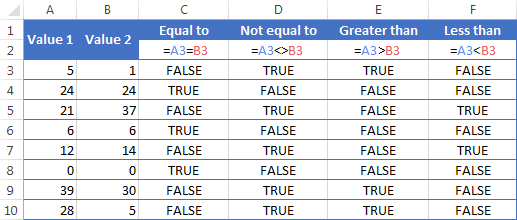
The screenshot below demonstrates the results returned by Equal to, Not equal to, Greater than and Less than logical operators:
It may seem that the above table covers it all and there's nothing more to talk about. But in fact, each logical operator has its own specificities and knowing them can help you harness the real power of Excel formulas.
Using "Equal to" logical operator in Excel
The Equal to logical operator (=) can be used to compare all data types - numbers, dates, text values, Booleans, as well as the results returned by other Excel formulas. For example:
| =A1=B1 | Returns TRUE if the values in cells A1 and B1 are the same, FALSE otherwise. |
| =A1="oranges" | Returns TRUE if cells A1 contain the word "oranges", FALSE otherwise. |
| =A1=TRUE | Returns TRUE if cells A1 contain the Boolean value TRUE, otherwise it returns FALSE. |
| =A1=(B1/2) | Returns TRUE if a number in cell A1 is equal to the quotient of the division of B1 by 2, FALSE otherwise. |
Example 1. Using the "Equal to" operator with dates
You might be surprised to know that the Equal to logical operator cannot compare dates as easily as numbers. For example, if the cells A1 and A2 contain the date "12/1/2014", the formula =A1=A2 will return TRUE exactly as it should.
However, if you try either =A1=12/1/2014 or =A1="12/1/2014" you will get FALSE as the result. A bit unexpected, eh?
The point is that Excel stores dates as numbers beginning with 1-Jan-1900, which is stored as 1. The date 12/1/2014 is stored as 41974. In the above formulas, Microsoft Excel interprets "12/1/2014" as a usual text string, and since "12/1/2014" is not equal to 41974, it returns FALSE.
To get the correct result, you must always wrap a date in the DATEVALUE function, like this =A1=DATEVALUE("12/1/2014")

Note. The DATEVALUE function needs to be used with other logical operator as well, as demonstrated in the examples that follow.
The same approach should be applied when you use Excel's equal to operator in the logical test of the IF function. You can find more info as well as a few formula examples in this tutorial: Using Excel IF function with dates.
Example 2. Using the "Equal to" operator with text values
Using Excel's Equal to operator with text values does not require any extra twists. The only thing you should keep in mind is that the Equal to logical operator in Excel is case-insensitive, meaning that case differences are ignored when comparing text values.
For example, if cell A1 contains the word "oranges" and cell B1 contains "Oranges", the formula =A1=B1 will return TRUE.
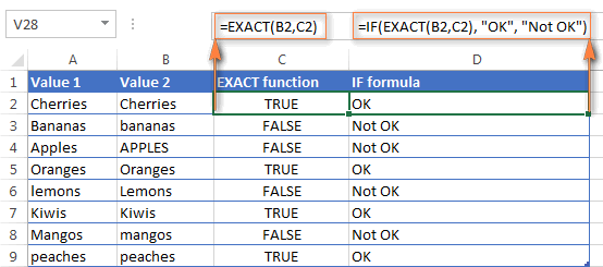
If you want to compare text values taking in to account their case differences, you should use the EXACT function instead of the Equal to operator. The syntax of the EXACT function is as simple as:
Where text 1 and text2 are the values you want to compare. If the values are exactly the same, including case, Excel returns TRUE; otherwise, it returns FALSE. You can also use the EXACT function in IF formulas when you need a case-sensitive comparison of text values, as shown in the below screenshot:
Note. If you want to compare the length of two text values, you can use the LEN function instead, for example =LEN(A2)=LEN(B2) or =LEN(A2)>=LEN(B2).
Example 3. Comparing Boolean values and numbers
There is a widespread opinion that in Microsoft Excel the Boolean value of TRUE always equates to 1 and FALSE to 0. However, this is only partially true, and the key word here is "always" or more precisely "not always" : )
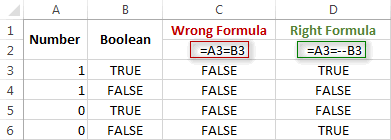
When writing an 'equal to' logical expression that compares a Boolean value and a number, you need to specifically point out for Excel that a non-numeric Boolean value should be treated as a number. You can do this by adding the double minus sign in front of a Boolean value or a cell reference, e. g. =A2=--TRUE or =A2=--B2.
The 1st minus sign, which is technically called the unary operator, coerces TRUE/FALSE to -1/0, respectively, and the second unary negates the values turning them into +1 and 0. This will probably be easier to understand looking at the following screenshot:
Note. You should add the double unary operator before a Boolean when using other logical operators such as not equal to, greater than or less than to correctly compare a numeric and Boolean values.
When using logical operators in complex formulas, you might also need to add the double unary before each logical expression that returns TRUE or FALSE as the result. Here's an example of such a formula: SUMPRODUCT and SUMIFS in Excel.
Using "Not equal to" logical operator in Excel
You use Excel's Not equal to operator (<>) when you want to make sure that a cell's value is not equal to a specified value. The use of the Not equal to operator is very similar to the use of Equal to that we discussed a moment ago.
The results returned by the Not equal to operator are analogous to the results produced by the Excel NOT function that reverses the value of its argument. The following table provides a few formula examples.
| Not equal to operator | NOT function | Description |
| =A1<>B1 | =NOT(A1=B1) | Returns TRUE if the values in cells A1 and B1 are not the same, FALSE otherwise. |
| =A1<>"oranges" | =NOT(A1="oranges") | Returns TRUE if cell A1 contains any value other than "oranges", FALSE if it contains "oranges" or "ORANGES" or "Oranges", etc. |
| =A1<>TRUE | =NOT(A1=TRUE) | Returns TRUE if cell A1 contains any value other than TRUE, FALSE otherwise. |
| =A1<>(B1/2) | =NOT(A1=B1/2) | Returns TRUE if a number in cell A1 is not equal to the quotient of the division of B1 by 2, FALSE otherwise. |
| =A1<>DATEVALUE("12/1/2014") | =NOT(A1=DATEVALUE("12/1/2014")) | Returns TRUE if A1 contains any value other than the date of 1-Dec-2014, regardless of the date format, FALSE otherwise. |
Greater than, less than, greater than or equal to, less than or equal to
You use these logical operators in Excel to check how one number compares to another. Microsoft Excel provides 4 comparison operates whose names are self-explanatory:
- Greater than (>)
- Greater than or equal to (>=)
- Less than (<)
- Less than or equal to (<=)
Most often, Excel comparison operators are used with numbers, date and time values. For example:
| =A1>20 | Returns TRUE if a number in cell A1 is greater than 20, FALSE otherwise. |
| =A1>=(B1/2) | Returns TRUE if a number in cell A1 is greater than or equal to the quotient of the division of B1 by 2, FALSE otherwise. |
| =A1<DATEVALUE("12/1/2014") | Returns TRUE if a date in cell A1 is less than 1-Dec-2014, FALSE otherwise. |
| =A1<=SUM(B1:D1) | Returns TRUE if a number in cell A1 is less than or equal to the sum of values in cells B1:D1, FALSE otherwise. |
Using Excel comparison operators with text values
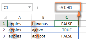
In theory, you can also use the greater than, greater than or equal to operators as well as their less than counterparts with text values. For example, if cell A1 contains "apples" and B1 contains "bananas", guess what the formula =A1>B1 will return? Congratulations to those who've staked on FALSE : )
When comparing text values, Microsoft Excel ignores their case and compares the values symbol by symbol, "a" being considered the lowest text value and "z" - the highest text value.
So, when comparing the values of "apples" (A1) and "bananas" (B1), Excel starts with their first letters "a" and "b", respectively, and since "b" is greater than "a", the formula =A1>B1 returns FALSE.
If the first letters are the same, then the 2nd letters are compared, if they happen to be identical too, then Excel gets to the 3rd, 4th letters and so on. For example, if A1 contained "apples" and B1 contained "agave", the formula =A1>B1 would return TRUE because "p" is greater than "g".
At first sight, the use of comparison operators with text values seems to have very little practical sense, but you never know what you might need in the future, so probably this knowledge will prove helpful to someone.
Common uses of logical operators in Excel
In real work, Excel logical operators are rarely used on their own. Agree, the Boolean values TRUE and FALSE they return, though very true (excuse the pun), are not very meaningful. To get more sensible results, you can use logical operators as part of Excel functions or conditional formatting rules, as demonstrated in the below examples.
1. Using logical operators in arguments of Excel functions
When it comes to logical operators, Excel is very permissive and allows using them in parameters of many functions. One of the most common uses is found in Excel IF function where the comparison operators can help to construct a logical test, and the IF formula will return an appropriate result depending on whether the test evaluates to TRUE or FALSE. For example:
=IF(A1>=B1, "OK", "Not OK")
This simple IF formula returns OK if a value in cell A1 is greater than or equal to a value in cell B1, "Not OK" otherwise.
And here's another example:
=IF(A1<>B1, SUM(A1:C1), "")
The formula compares the values in cells A1 and B1, and if A1 is not equal to B1, the sum of values in cells A1:C1 is returned, an empty string otherwise.
Excel logical operators are also widely used in special IF functions such as SUMIF, COUNTIF, AVERAGEIF and their plural counterparts that return a result based on a certain condition or multiple conditions.
You can find a wealth of formula examples in the following tutorials:
2. Using Excel logical operators in mathematical calculations
Of course, Excel functions are very powerful, but you don't always have to use them to achieve the desired result. For example, the results returned by the following two formulas are identical:
IF function: =IF(B2>C2, B2*10, B2*5)
Formula with logical operators: =(B2>C2)*(B2*10)+(B2<=C2)*(B2*5)
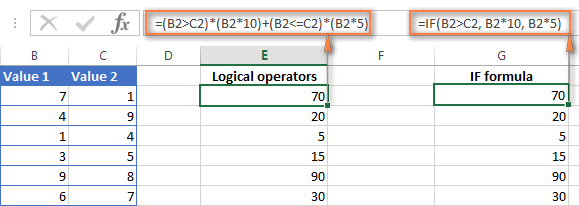
I guess the IF formula is easier to interpret, right? It tells Excel to multiply a value in cell B2 by 10 if B2 is greater than C2, otherwise the value in B1 is multiplied by 5.
Now, let's analyze what the 2nd formula with the greater than and less than or equal to logical operators does. It helps to know that in mathematical calculations Excel does equate the Boolean value TRUE to 1, and FALSE to 0. Keeping this in mind, let's see what each of the logical expressions actually returns.
If a value in cell B2 is greater than a value in C2, then the expression B2>C2 is TRUE, and consequently equal to 1. On the other hand, B2<=C2 is FALSE and equal to 0. So, given that B2>C2, our formula undergoes the following transformation:
![]()
Since any number multiplied by zero gives zero, we can cast away the second part of the formula after the plus sign. And because any number multiplied by 1 is that number, our complex formula turns into a simple =B2*10 that returns the product of multiplying B2 by 10, which is exactly what the above IF formula does : )
Obviously, if a value in cell B2 is less than in C2, then the expression B2>C2 evaluates to FALSE (0) and B2<=C2 to TRUE (1), meaning that the reverse of the described above will occur.
3. Logical operators in Excel conditional formatting
Another common use of logical operators is found in Excel Conditional Formatting that lets you quickly highlight the most important information in a spreadsheet.
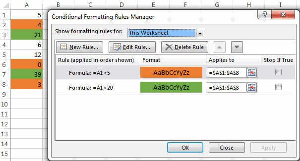
For example, the following simple rules highlight selected cells or entire rows in your worksheet depending on a value in column A:
Less than (orange): =A1<5
Greater than (green): =A1>20
For the detailed-step-by-step instructions and rule examples, please see the following articles:
As you see, the use of logical operators in Excel is intuitive and easy. In the next article, we are going to learn the nuts and bolts of Excel logical functions that allow performing more than one comparison in a formula. Please stay tuned and thank you for reading!
 by
by
1252 comments
I need help with figuring out and writing a formula. I have data in column A that is also in columns K,M,P,R depending on the department it belongs too. I want to be able to delete something in column A and have it also remove the data in the other column and either leave the cell blank or highlight it. I'm not sure where to even begin. I've tried searching for what I need but can't find the exact formula I need. It seems like I may need two formulas? I appreciate any and all help/guidance. Thanks in advance!!!!!
Hi! You can delete data that is written in a cell either manually or by using a VBA macro. It is impossible to do it with a formula. I'm not quite sure what criteria you want to use to highlight a cell. But maybe this article will be helpful: Excel conditional formatting formulas based on another cell.
Sir
I am recording wind direction as N,S,E,W, NE,NNE etc. and same has to be converted to a code number like 36,02,05,07,14 etc. How it possible to convert the text to numbers in Excel?
Please help me
Hi! You can use a nested IF function. For example:
=IF(A1="N",36,IF(A1="S",2,""))
For detailed instructions and examples, and other methods, click here: Excel Nested IF statement: examples, best practices and alternatives.
Hi how are u doin,
I want to put percentages looks like (100%,90%,80% until 10%) and i want it works like that, if the product lower then 1$ then add 100% price, if its 3% add 90% until the 10%
can anyone tell me how to do that please?
Hi! Unfortunately, the conditions you described are not clear. If you have a lot of calculations on conditions, I recommend using the IFS function. Multiplication by percent is described in detail in this article: How to calculate percentage in Excel - formula examples.
what is the formula of number is greater than zero is equal to zero
Hi! Look for the example formulas here: IF function in Excel: formula examples for text, numbers, dates, blanks.
-if(K5=" ",50,0,if(L5=" ",50,0,if(M5=" ",50,0,if(N5=" ",50,0,if(O5=" ",50,0,if(P5=" ",50,0,If(Q5=" ",50,0,if(R5=" ",50,0,if(S5=" ",50,0,if(T5=" ",50,0,if(U5=" ",50,0,if(V5=" ",50,0,if(W5=" ",50,0,if(X5=" ",50,0,if(Y5=" ",50,0))))))))))))))
System replies I've entered too many arguments for this function, but I am in 365 and I thought the number of arguments was 67. I have 29. What I am trying to arrive at a person gets a $50 bonus in another column if the person has not rec'd any marks in cells K→Y, if there is an x in any of those cells they lose the $50 bonus.
Hi! You can find the examples and detailed instructions here: Nested IF in Excel – formula with multiple conditions. Your IF function has four arguments instead of three: if(K5=" ", 50, 0, if(
Your formula is difficult to understand, but it may be correct to remove 0 : if(K5=" ",50,if(......
I’m trying to get a formula to work and not having any luck. Can someone assist?
I need to say
if B5=PJJ and H5>0 then add 100+I5*3+M5… if B5PJJ and H5>0 then 100+I5*3+M5+O5 also if I can add to this line that if H5=0 then L5+N5/2
I got it to work without the AND saying just IF(H5>0,100+I5*3+M5+O5,IF(H5=0,(L5+N5)/2)) but when I add the B5 into the mix, I can’t get it to work.
I noticed a type, where I have B5PJJ that should say B5PJJ
If we want to add to the confusion, I’d love to get G5 involved too but I might be pushing it.
Ultimately if G5 is N all the prior stuff is true. But if G5=Y then I need to change the multiplier to 4.5 instead of 3
Apparently it doesn’t like the not equal to symbols for some reason, I’ve put them twice and they don’t seem to take. B5 is not equal to PJJ
Hi! You've further confused your description of the problem.
Hi! Look for the example formulas here: IF AND in Excel: nested formula, multiple statements, and more. You may be getting an error because PJJ is an invalid cell reference.
how can i use data validation custom to formulate a formula to put a value on a A1 that is greater than in A2. And A2 that is less than in A1
Hi! Try to use the recommendations described in this guide: How to create custom data validation with formula.
A1 > A2
Hi Can you pls help me make the formula
IF function..
A1> 15% Major ,
A1 < = 15% Minor
A1 = 0 is Neutral
Cell A1 is greater than 15% is Major, Lesser than or equal to 15% Minor, and Zero is Neutral
Hi! Look for the example formulas here: Nested IF in Excel – formula with multiple conditions.
Hello,
If i have value in cell A1, that can vary and is SUM of other cells A2:A10, how do i set up my function in C1 to do the following :
If value in A1 is from 0-50000 show value from B1,
If value in A1 is from 51000-100000 show value from B2,
If value in A1 is from 101000-150000 show value from B3,
Etc etc... Thanks!!
Hi! For how to make a choice based on multiple criteria, see the examples in this article: Nested IF in Excel – formula with multiple conditions.
Hi, can anyone help me?
i have a range below.
any value entered in A1 will result to the range below.
ex.
if i input 2300 the value will be multiplied to 2%
but if i put 6000 the output will be just "100"
1000-1500 ; (multiplied by) 0.01 of 1%
1500-4999 ; (multipled by) 0.2 of 2%)
4999-99999 ; the return value is plain "100".
I'm not quite sure how to formulate it but i keep getting error on my formula.
hope someone will help
Hi! The following tutorial should help: Excel Nested IF statements - examples, best practices and alternatives.
Hope This formula will help you!
=IF(AND(B1>1000,B11500,B15000,B1<10000),B1*0.3,0)))
COL A COL B
Result 6000
Output 1800
Paste the formula in column b2 and enter the value in column b1.
SN Name Designation Subject Code Seniority No. of times taught
A B C D E F
1 Dr. M.Chandra Sekhar Professor A3CIT201 3 5
2 Mr. P.L.N.Raju Associate Professor A3CIT201 4 4
3 Mr. K.V.Subba Raju Associate Professor A3CIT201 3 6
4 Mr. G. Ramakumar Assistant Professor A3CYT101 2 6
5 Dr. GVSR Pavan Kumar Associate Professor A3CYT101 3 6
6 Dr. Abdul Rajack Professor A3CYT101 1 6
7 Mr.KVV Prasad Associate Professor A3EET201 2 4
8 Dr.Yoganandh Patnaik Assistant Professor A3EET201 5 3
9 Mr.G. Sankar Mani Professor A3EET201 3 4
10 Mr.SMK Patnaik Professor A3EET201 7 5
11 Mr.K.S.Ravi kumar Assistant Professor A3EET201 2 3
12 Mr.D.Rajesh Assistant Professor A3EET201 8 4
13 Dr.B.M.B.Krushna Professor A3MAT102 1 4
14 Dr.S.Atchuta Rao Professor A3MAT103 1 4
15 Dr. M. Sivaram Prasad Professor A3PYT101 2 4
16 Dr. BBVS Vara Prasad Assistant Professor A3PYT101 3 4
17 Dr. G. Srinivasa Reddy Associate Professor A3PYT101 1 4
18 Mr. P. Sateesh Professor A3PYT102 1 5
19 Dr. BBVS Vara Prasad Assistant Professor A3PYT102 3 4
20 Dr. M. Sivaram Prasad Associate Professor A3PYT102 4 5
21 A3CIT201
How to define formula in above table with the below multiple conditions
1. Maximum value of f column
2. D column value = b21
3. C column value = “professor”, or “associate professor” or “senior assistant professor” or “assistant professor”
4. Maximum e column value = maximum value consider (same value in c column i.e. “professor”)
5. Final b column value show
Hi! Not all of your conditions are clear, but I can recommend the following:
1. F1=MAX(F1:F100) Read more: Excel MAX function - formula examples to find highest value
2. D1=$B$21
3. =ISNUMBER(SEARCH("professor",C1)) Read more: How to find substring in Excel
Use this in the IF AND formula and copy down the column.
Hi
Not sure if anyone can help I am trying to write an if formula were if k2 = "Contractual" I want excel to return BL2+BL2*9 and if K2 dosen't = "Contractual" I want excel to return BM2/3*12. The formula that I have written is
=IFS(K2="Contractual",BL2+BJ2*9,K2=NOT(K2="Contractual"),BM2/3*12)
For some reason I just can't get it to work - any ideas?
Thanks :-)
Hi! I can't verify your formula, as I don't have your data. Check the cell references. You can also write it using the IF function:
=IF(K2="Contractual",BL2+BJ2*9,BM2/3*12)
Hi Alexander,
I am looking for "90%" value as end result.
Data has
Specialty 10% 40% 90%
PA: Physiatry $55,418 $57,546 $59,230
PA: Psychiatry $107,767 $108,228 $108,576
PA: Pulmonary $98,960 $99,886 $101,238
PA: Rheumatology $88,429 $90,045 $91,529
Cell A1 has Specialty (Ex: PA : Psychiatry)
Cell B1 has salary (Ex: 100,000) (Note: This keeps changing every month as the value shows the paid amount)
Cell C3 needs result as (B1 values fall under one of the % from data, if values are not range it has to give me result as "90%" )
Thanks!
Hi! Unfortunately, I cannot understand what you want to do. In your example, cell C3 already contains data 108228. Please explain it in more detail.
I'm so close, but can't quite get there!
I have a cell [F3], and if the number in that cell is 5 or higher, than I would like one value in another cell copied [W11].
If the number in that cell is less than 5, than I would like the value from a different cell copied [W10}.
=IF(OR(F3>=5,F3<5),$W$11,$W$10)
W10 and W11 are both totally separate calculations.
Don't think it matters, but W12 is where the value is to be displayed.
Please help and thank you in advance.
Hi! I recommend that you study the instructions for the IF function carefully: IF function in Excel: formula examples for text, numbers, dates, blanks.
=IF(F3>=5,$W$11,$W$10)
Hello -- I am working with the following:
1) Column of data that contains parent account numbers. These values could be used once or could be the same parent in multiple rows.
2) Column of processor names associated with each parent number.
3) Column of open dollars in each row.
Challenge to solve:
1) I need to populate the same processor name for each unique parent number, utlizing the existing processor with the largest open dollars.
My spreadsheet is over 100,000 rows so I'm looking for a formula to help me accomplish this. I have Windows 365.
Hi! To understand what you want to do, give an example of the source data and the expected result.
A1 B1
15001 *
* here i need the formula: A1 greater that 15000=15000, A1 equal to 15000=15000 and A1 less than 15000=A1
with regards.
Hi!
Try to follow the recommendations from this article: Excel IF function with multiple conditions.
I need the same type of function - i was not able to get what i needed from the link above - any other assistance?
Unfortunately, I can't guess what you want.
if A2 =100 and less than 200, and a2 is >=200 then a1*2.5/100 kindly help to find this formula
Hi! Your terms are contradictory and cannot be used in an IF formula. Here is the article that may be helpful to you: Excel IF function with multiple conditions.
Hello! my data is
December November October September August July June May April March February January Need to monitor?
515,100,000 515,100,000 676,700,000 515,100,000 515,100,000 353,500,000 353,500,000 353,500,000 200,000,000 - 353,500,000 - No
is there any formula so the condition in NEED TO MONITOR is Based on IF Values in November and so on is greater than December then its No if its lesser than december then its yes. thank you !
Hi!
If I understand your task correctly, the following tutorial should help: Excel IF between two numbers or dates.
I have a spreadsheet in ‘Numbers Mac’ & I reckon it’s quite similar to Excel. I really need your expertiseto help me solve the question below.
I would like to use a formula to find the tidal window (start & end date with time) from the Tide Table below base on Vsl Eta & Height of Tide Required.
Eg:- ‘CELL ETA’ : 02 Jan 2023 @ 19:00 ‘“CELL HOT REQUIRED”: 2.8
Extract from the tide table as below:-
A B C D E F G H I J K L M N O P Q R S T U V W X Y
1. Date / Time 00 01 02 03 04 05 06 07 08 09 10 11 12 13 14 15 16 17 18 19 20 21 22 23
2. 01 Jan 2023 3.8 3.8 3.6 3.3 2.8 2.4 2.0 1.9 1.9 2.0 2.4 2.7 3.0 3.1 3.1 3.1 2.9 2.6 2.3 2.0 1.9 2.0 2.3 2.7
3. 02 Jan 2023 2.8 2.9 3.1 3.3 3.4 3.2 3.0 2.7 2.6 2.3 2.0 1.7 1.0 1.3 1.2 1.1 2.2 3.0 3.2 3.0 2.8 2.6 2.7 2.5
4. 03 Jan 2023 2.8 3.7 3.8 3.6 3.3 3.0 2.6 2.0 1.7 1.7 1.9 2.2 2.6 2.9 3.0 3.2 3.2 3.1 2.8 2.1 2.1 1.9 1.9 2.2
5. 04 Jan 2023 2.3 2.3 2.5 2.7 3.0 2.9 2.8 2.9 2.7 2.3 2.1 2.1 1.8 1.7 1.5 1.8 2.0 2.2 2.4 2.5 2.5 2.6 3.0 3.0
Base on vsl Eta 02nd Jan 2023 @ 19:00 the HOT is 3.0m from the table above (by using formula Index & Match). As per calculation in my spreadsheet, she only required 2.8m in order to pass safely the critical area or shallow water. So anything above or equal to 2.8m is considered as safe tidal window for her to pass. Usually we provide the vsl with 2 tidal window just in case she had been delayed or misss the present window. . Do note that in certain day, there are two tidal window but should provide her the nearest window as per her ETA. It can be either before or after the ETA. Whichever nearest to her ETA is known as ‘PRESENT WINDOW’ and the following window is known as ‘NEXT WINDOW’
Question:-
What formula or how to have a formula input into a particular cell based on Vsl ETA & Height of Tide Required in order to get the tidal window/range ( start date & time to end date & time. How to let the formula pick up the window which is closest or nearest to the Vsl Eta? Or is it necessary to breakdown the formula into a couple of cell before getting the correct answer?
One formula for the ‘PRESENT WINDOW’ another formula for ‘NEXT WINDOW’. ( The formula can be either start & end in one cell or they can also be separate).
The answer is as follows:-
Present window: 02nd/1700 to 02nd/2000
Next window: 03rd/0000 to 03rd/0530 ( is it possible to include interpolation in the formula too )
Thank you in advance.
SID
Hi!
To search for values or set a filter, the data must be arranged by rows, not by columns. Your request goes beyond the advice we provide on this blog. This is a complex solution that cannot be found with a single formula. If you have a specific question about the operation of a function or formula, I will try to answer it.
Hiya,
I am looking for a formula to show the following:
Looking at the sum of a cell (cell A). If its less than zero, return 0. But if its greater than 0, return the value of said cell (cell A), but capped at a maximum 1,000 (or x number).
Could someone kindly provide the formula for this. I can't work it out.
thank you in advance.
Hi!
To show a value by two conditions, use the nested IF function.
=IF(A2<0,0,IF(A2>1000,1000,""))
Or use MIN and MAX function
=MIN(MAX(0,A2),1000)
I hope it’ll be helpful.
Hi, I am looking for a formula to skip going through a pivot table.
I am looking for MAX SUM OF KM PER DAY (or max km done per day), when there can be multiple entries for a given day.
Ex.
2023-01-01 5
2023-01-01 5
2023-01-01 10
2023-01-02 10
2023-01-03 8
2023-01-04 18
Thank you !
(Here the result would yield : 20, since the max sum per day is on 2023-01-01, 5 + 5 + 10)
Hi!
To find the amount for a certain day, maybe you can use the SUMIF function.
Hi!
Based on your description, it is hard to completely understand your task. However, I’ll try to guess and offer you the following guide: Excel MAX IF formula to find largest value with conditions.
i want you to know how a formula is done for,
if C26 is equal to 1, the result should be whichever is less in both amounts of 12.5% of E22 and 20,000/- , otherwise NIL.
I'm trying to make a formula for (if d3 is equal to or less that 10,000 then E3 is 0, if d3 is between 10,001-20,000 then E3 is 50, if d3 is between 20,001-30,000 then E3 is 100, if d3 is between 30,001-40,000 then e3 is 150, if d3 is greater than 40,001 then e3 is 200)
Hi!
See an example of solving such a problem here: Excel Nested IF statement.
i need a formula to calculate wages over 7000 and wages under 7000. and would like to show the amount over or under in a cell
Hi!
Here is the article that may be helpful to you: IF function in Excel: formula examples for text, numbers, dates, blanks.
how do you write this in an IF statement:
IF D2 is 31 then B2*75
=IF(B2=31,B2*75)
Hi
if a row have alphabets like a code A,B,C,UR. i need a final result in another column A<B<C<UR.
is this possible
Hi!
Have you tried the ways described in this blog post? If they don’t work for you, then please describe your task in detail. As it's currently written, it's hard to tell exactly what you're asking.
Hello, great information, thank you.
Is there a logical operator for [="unique value" in a column] is unique in a column?
Ultimately what I'm trying to do is create an include for the filter function and I want to reference a column in the filter function array and, along with a few other filters, only return unique values.
Hi!
Your question is not very clear to me, but perhaps you will find this information useful: Unique values based on multiple criteria. If this is not what you wanted, please describe the problem in more detail.