The tutorial shows how to use IF together with the AND function in Excel to check multiple conditions in one formula.
Some things in the world are finite. Others are infinite, and the IF function seems to be one of such things. On our blog, we already have a handful of Excel IF tutorials and still discover new uses every day. Today, we are going to look at how you can use IF together with the AND function to evaluate two or more conditions at the same time.
IF AND statement in Excel
In order to build the IF AND statement, you obviously need to combine the IF and AND functions in one formula. Here's how:
Translated into plain English, the formula reads as follows: IF condition 1 is true AND condition 2 is true, do one thing, otherwise do something else.
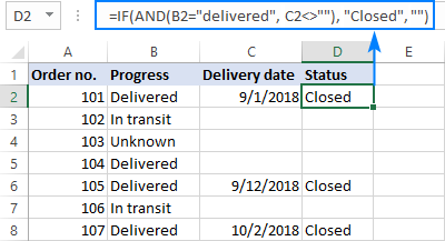
As an example, let's make a formula that checks if B2 is "delivered" and C2 is not empty, and depending on the results, does one of the following:
- If both conditions are TRUE, mark the order as "Closed".
- If either condition is FALSE or both are FALSE, then return an empty string ("").
=IF(AND(B2="delivered", C2<>""), "Closed", "")
The screenshot below shows the IF AND function in Excel:
If you'd like to return some value in case the logical test evaluates to FALSE, supply that value in the value_if_false argument. For example:
=IF(AND(B2="delivered", C2<>""), "Closed", "Open")
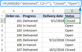
The modified formula outputs "Closed" if column B is "delivered" and C has any date in it (non-blank). In all other cases, it returns "Open":
Note. When using an IF AND formula in Excel to evaluate text conditions, please keep in mind that lowercase and uppercase are treated as the same character. If you are looking for a case-sensitive IF AND formula, wrap one or more arguments of AND into the EXACT function as it is done in the linked example.
Now that you know the syntax of the Excel IF AND statement, let me show you what kind of tasks it can solve.
Excel IF: greater than AND less than
In the previous example, we were testing two conditions in two different cells. But sometimes you may need to run two or more tests on the same cell. A typical example is checking if a cell value is between two numbers. The Excel IF AND function can easily do that too!
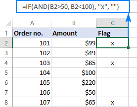
Let's say you have some sales numbers in column B and you are requested to flag the amounts greater than $50 but less than $100. To have it done, insert this formula in C2 and then copy it down the column:
=IF(AND(B2>50, B2<100), "x", "")
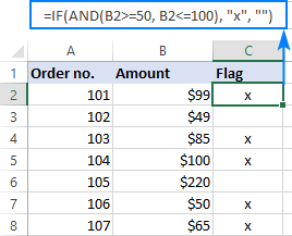
If you need to include the boundary values (50 and 100), use the less than or equal to operator (<=) and greater than or equal to (>=) operator:
=IF(AND(B2>=50, B2<=100), "x", "")
To process some other boundary values without changing the formula, enter the minimum and maximum numbers in two separate cells and refer to those cells in your formula. For the formula to work correctly in all the rows, be sure to use absolute references for the boundary cells ($F$1 and $F$2 in our case):
=IF(AND(B2>=$F$1, B2<=$F$2), "x", "")
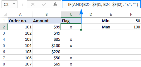
By using a similar formula, you can check if a date falls within a specified range.
For example, let's flag dates between 10-Sep-2018 and 30-Sep-2018, inclusive. A small hurdle is that dates cannot be supplied to the logical tests directly. For Excel to understand the dates, they should be enclosed in the DATEVALUE function, like this:
=IF(AND(B2>=DATEVALUE("9/10/2018"), B2<=DATEVALUE("9/30/2018")), "x", "")
Or simply input the From and To dates in two cells ($F$1 and $F$2 in this example) and "pull" them from those cells by using the already familiar IF AND formula:
=IF(AND(B2>=$F$1, B2<=$F$2), "x", "")
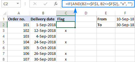
For more information, please see Excel IF statement between two numbers or dates.
IF this AND that, then calculate something
Apart from returning predefined values, the Excel IF AND function can also perform different calculations depending on whether the specified conditions are TRUE or FALSE.
To demonstrate the approach, we will be calculating a bonus of 5% for "Closed" sales with the amount greater than or equal to $100.
Assuming the amount is in column B and the order status in column C, the formula goes as follows:
=IF(AND(B2>=100, C2="closed"), B2*10%, 0)
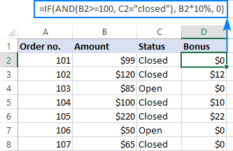
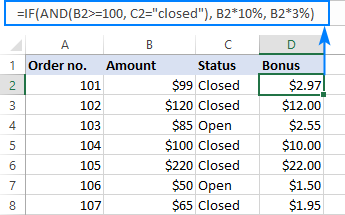
The above formula assigns zero to the rest of the orders (value_if_false = 0). If you are willing to give a small stimulating bonus, say 3%, to orders that do not meet the conditions, include the corresponding equation in the value_if_false argument:
=IF(AND(B2>=100, C2="closed"), B2*10%, B2*3%)
Multiple IF AND statements in Excel
As you may have noticed, we have evaluated only two criteria in all the above examples. But there is nothing that would prevent you from including three and more tests in your IF AND formulas as long as they comply with these general limitations of Excel:
- In Excel 2007 and higher, up to 255 arguments can be used in a formula, with a total formula length not exceeding 8,192 characters.
- In Excel 2003 and lower, no more than 30 arguments are allowed, with a total length not exceeding 1,024 characters.
As an example of multiple AND conditions, please consider these ones:
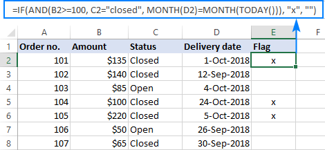
- Amount (B2) should be greater than or equal to $100
- Order status (C2) is "Closed"
- Delivery date (D2) is within the current month
Now, we need an IF AND statement to identify the orders for which all 3 conditions are TRUE. And here it is:
=IF(AND(B2>=100, C2="Closed", MONTH(D2)=MONTH(TODAY())), "x", "")
Given that the 'current month' at the moment of writing was October, the formula delivers the below results:
Nested IF AND statements
When working with large worksheets, chances are that you may be required to check a few sets of different AND criteria at a time. For this, you take a classic Excel nested IF formula and extend its logical tests with AND statements, like this:
To get the general idea, please look at the following example.
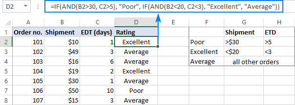
Supposing you want to rate your service based on the shipment cost and estimated time of delivery (ETD):
- Excellent: shipment cost under $20 and ETD under 3 days
- Poor: shipment cost over $30 and ETD over 5 days
- Average: anything in between
To get it done, you write two individual IF AND statements:
IF(AND(B2<20, C2<3), "Excellent", …)
IF(AND(B2>30, C2>5), "Poor", …)
…and nest one into the other:
=IF(AND(B2>30, C2>5), "Poor", IF(AND(B2<20, C2<3), "Excellent", "Average"))
The result will look similar to this:
More formula examples can be found in Excel nested IF AND statements.
Case-sensitive IF AND function in Excel
As mentioned in the beginning of this tutorial, Excel IF AND formulas do not distinguish between uppercase and lowercase characters because the AND function is case-insensitive by nature.
If you are working with case-sensitive data and want to evaluate AND conditions taking into account the text case, do each individual logical test inside the EXACT function and nest those functions into your AND statement:
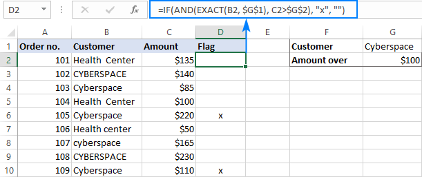
For this example, we are going to flag orders of a specific customer (e.g. the company named Cyberspace) with an amount exceeding a certain number, say $100.
As you can see in the below screenshot, some company names in column B look the same excerpt the characters case, and nevertheless they are different companies, so we have to check the names exactly. The amounts in column C are numbers, and we run a regular "greater than" test for them:
=IF(AND(EXACT(B2, "Cyberspace"), C2>100), "x", "")
To make the formula more flexible, you can input the target customer name and amount in two separate cells and refer to those cells. Just remember to lock the cell references with $ sign ($G$1 and $G$2 in our case) so they won't change when you copy the formula to other rows:
=IF(AND(EXACT(B2, $G$1), C2>$G$2), "x", "")
Now, you can type any name and amount in the referenced cells, and the formula will flag the corresponding orders in your table:
IF OR AND formula in Excel
In Excel IF formulas, you are not limited to using only one logical function. To check various combinations of multiple conditions, you are free to combine the IF, AND, OR and other functions to run the required logical tests. Here is an example of IF AND OR formula that tests a couple of OR conditions within AND. And now, I will show you how you can do two or more AND tests within the OR function.
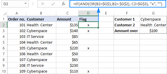
Supposing, you wish to mark the orders of two customers with an amount greater than a certain number, say $100.
In the Excel language, our conditions are expressed in this way:
OR(AND(Customer1, Amount>100), AND(Customer2, Amount>100)
Assuming the customer names are in column B, amounts in column C, the 2 target names are in G1 and G2, and the target amount is in G3, you use this formula to mark the corresponding orders with "x":
=IF(OR(AND(B2=$G$1, C2>$G$3), AND(B2=$G$2, C2>$G$3)), "x", "")
The same results can be achieved with a more compact syntax:
=IF(AND(OR(B2=$G$1,B2= $G$2), C2>$G$3), "x", "")
Not sure you totally understand the formula's logic? More information can be found in Excel IF with multiple AND/OR conditions.
That's how you use the IF and AND functions together in Excel. Thank you for reading and see you next week!
Practice workbook
IF AND Excel – formula examples (.xlsx file)
 by
by
475 comments
Would you be able to tell from the below formula why this isn't working?
Right now, I am trying to pull data based on description (5 total | 5 rows) in column A and the month in row 38 starting in column B (Jan-Dec). Basically a 5 x 12 grid.
My formula is puling all is pulling all "None".
Are there limitations to the formula where it won't pull across row and columns?
=IF(AND($C$4:$C$32=$A39,$H$4:$H$32=B$38),"X","None")
Hi! Sorry, it's not quite clear what you are trying to achieve. Your description of the problem does not match the formula. From column C to column H and from row 4 to row 32 is not a 5 x 12 grid. Please clarify your specific problem or provide additional details to highlight exactly what you need.
Reached that point of frustration... Can't see what I'm doing wrong here :-(
This is trying to test for any of the words, 'Health, Performance or Conduct' being in N105,
AND
the number of comma-separated strings in V105 being either 'two or more' or otherwise 'one'.
=IF(AND
IF(OR(N105="Health",N105="Performance",N105="Conduct"),
IF((LEN(V105)-LEN(SUBSTITUTE(V105,",",""))+1)>1)),"Two+", "One")
Help greatly appreciated
Hi! I’m sorry, but your description doesn’t give me a complete understanding of your task. Maybe this article will be helpful: How to find substring in Excel. To give better advice, give an example of the value in N105 and the desired result.
Thank you, Alexander.
N105 will have one of the values of "Health", "Performance", "Conduct", "Suitability" or "Prohibited".
V105 will have one or more comma-separated free-text strings.
Some examples of the results I'm seeking:
1. N105 = "Health" and V105 = "Treatment program, Approved clinic, Education" returns result of "Two+"
2. N105 = "Health" and V105 = "Drug testing" returns result of "One"
3. N105 = "Conduct" and V105 = "Supervision, Education" returns result of "Two+"
4. N105 = "Prohibited" and V105 = "Suspended" returns result a FALSE result
I realise that I think I haven't resolved the FALSe part of the problem as in example 4.
Thanks for any help
Hi! I'm not sure if I understood you correctly. The description you provided is not entirely clear. However, it seems to me that the formula below will work for you:
=IF(AND(OR(N105="Health",N105="Performance",N105="Conduct"),
(LEN(V105)-LEN(SUBSTITUTE(V105,",",""))+1)>1),"Two+", IF(AND(OR(N105="Health",N105="Performance",N105="Conduct"),
(LEN(V105)-LEN(SUBSTITUTE(V105,",",""))+1)=1), "One"))
I recommend reading this guide: Nested IF with OR/AND conditions.
Thank you again, Alexander. That has done the trick! Really appreciate the help :-)
I have the following scenario and can't quite get all the nests. Hope you can help.
I need it to work like this:
IF Sheet1 B9:B20 match any of Sheet 2 B9:20 THEN add Sheet 2 K9:K20 and bring that value back to the cell with the formula
hi! Based on your description, it is hard to completely understand your task. I can assume that you can use the INDEX MATCH functions to find a value in a range. If this does not help, explain the problem in detail.
I am placing/writing a formula in cell C1
In A1 - Its EXPIRY DATE
In B1 - Its RENEWAL DATE
=IF(TODAY()>=B1,"SEND RENEW REMINDER","WAIT")
The above formula is working.
Now, I want to apply one more condition in same cell C1 - That if A1 is less than TODAY's date, the result should be "PENDING" and if I write manually (CANCELLED) in A1, the result should be "CANCELLED". Something like =IF(TODAY()<A1,"PENDING") =IF(A1=CANCELLED,"CANCELLED")
I am finding difficulty to apply the second condition merging with first condition in the same cell.
Please help me out.
Hi! To write multiple conditions in an IF formula, you can use this guide: Nested IF in Excel – formula with multiple conditions. For example:
=IF(TODAY()<A1,"PENDING", IF(TODAY()>=B1,"SEND RENEW REMINDER","WAIT"))
=IF(AND(F2="",G2=""),SUMIF(Budget!$B:$B,'One Pager'!$L$2,Budget!$U:$U),IF(F2="",SUMIF(Budget!$C:$C,'One Pager'!$L$2,Budget!$U:$U))),IF(AND(E2="",G2=""),SUMIF(Budget!$D:$D,'One Pager'!$L$2,Budget!$U:$U),IF(E2="",SUMIF(Budget!$E:$E,'One Pager'!$L$2,Budget!$U:$U))),IF(AND(D2="",G2=""),SUMIF(Budget!$F:$F,'One Pager'!$L$2,Budget!$U:$U),IF(D2="",SUMIF(Budget!$G:$G,'One Pager'!$L$2,Budget!$U:$U))),IF(AND(C2="Axis bank",G2=""),SUMIF(Budget!$H:$H,'One Pager'!$L$2,Budget!$U:$U),IF(C2="Axis bank",SUMIF(Budget!$I:$I,'One Pager'!$L$2,Budget!$U:$U)))
showing #value error
Hi! It is very difficult to understand a formula that contains unique references to your workbook worksheets. Hence, I cannot check its work, sorry.
I recommend reading this guide: #VALUE error in Excel: causes and fixes.
how to set an excel formula wherein,
i have a range between 5-11, if i input a value between 5-11, the 6% will appear automatically but if i input below or above the range, answer will be negative below or above 6%
Hi! Based on your description, it is hard to completely understand your task. Use these instructions to check a number within a specified interval: Excel IF: greater than AND less than. For example:
=IF(AND(A2>5, A2<11), 6%, "")
What is Wrong with this formula, it is giving ERROR:
IF(AND(N15="ACRE",P15="BIGHA”),M15*3.02500,IF(AND(N15="ACRE",P15="KATHA”),M15*60.50000,IF(AND(N15="KATHA",P15="ACRE”),M15*0.01653,IF(AND(N15="BIGHA",P15="ACRE”),M15*0.33058,IF(AND(N15="KATHA",P15="SQ.FT.”),M15*720.00003,IF(AND(N15="KATHA",P15="CHHATAK”),M15*16.00000,IF(AND(N15="CHHATAK",P15="KATHA”),M15*0.06250,IF(AND(N15="KATHA",P15="DECIMAL”),M15*1.65289256,IF(AND(N15="DECIMAL",P15="KATHA”),M15*0.60500,IF(AND(N15="ACRE",P15="SQ.FT.”,M15*43560,IF(AND(N15="SQ.FT.",P15="ACRE”,M1/43560)))))))))))
Hi! Check the quotation marks in your formula. Use " instead of ”
I made a grade monitoring sheet with 9 subjects I made 1 formula , I want to make a formula where the final grade will show in the table if I type the number or subject .For example 1 = SUBJECT 1.. this is my formula =IF(A1=1,W12) ..W12 is the final grade.. then in the next row I the formula I made is =IF(A1=2,W12)... it's shows the correct grade but the first column become FALSE.. what should I do?
Hi! Only one value can be written in cell A1. In this case, it is either 1 or 2. So one of your formulas will always return FALSE. Unfortunately, I don't quite understand what result you want to get. Maybe this article will be helpful: Nested IF in Excel – formula with multiple conditions.
Hello - I am trying to calculate increased or decreased spend YoY based on current performance. Here is the logic: (1) if rev is up and spend is down, increase spend by % growth in rev (2) if rev is down and spend is up, decrease spend by % decline in rev (3) if rev is up and spend is up, increase spend by % increase in rev (4) if rev and spend are flat, keep spend as is. The data inputs are across multiple sheets.
The tab names are (1) US YoY Spend % Change (2) US Rev YoY % Change (3) US Publisher Net Spend by Month
Here is the formula I'm inputting. I keep running into errors:
=IF(AND('US YoY Spend % Change'!$S$3>0%,'US Rev YoY % Change'!$S$3<0%),'US Publisher Net Spend by Month'!F3+(‘US Publisher Net Spend by Month'!F3*'US Rev YoY % Change'!S3),IF(AND('US YoY Spend % Change'!$S$30%),'US Publisher Net Spend by Month'!F3+(‘US Publisher Net Spend by Month'!F3*'US Rev YoY % Change'!S3),IF(AND('US YoY Spend % Change'!$S$3>0%,'US Rev YoY % Change'!$S$30>0%),'US Publisher Net Spend by Month'!F3+('US Publisher Net Spend by Month'!F3*'US Rev YoY % Change'!S3),IF(AND('US YoY Spend % Change'!$S$3=0%,'US Rev YoY % Change'!$S$30=0%),'US Publisher Net Spend by Month'!F3, ‘US Publisher Net Spend by Month'!F3))))
Looking for some guidance please..
I have 3 IF formulas - all functioning as i need them to in separate cells. however i am struggling to nest them. For context i am creating a diary that will flag up dates for various conditions.
the 3 formulas are as follows :
1- =IF(H2>=TODAY()+8,"OVER 7 DAYS", "")
2- =IF(AND(H2>=TODAY()+1,H2<=TODAY()+7),"WITHIN 7 DAYS","")
3- =IF(H2=TODAY()+8),"OVER 7 DAYS", IF(AND(H2>=TODAY()+1),(H2<=TODAY()+7)),"WITHIN 7 DAYS", IF((H2=TODAY()+8),"OVER A WEEK", (H2>=TODAY()+1 & H2<=TODAY()+7), "WITHIN 7 DAYS" , (H2<=TODAY()), "TODAY / OVERDUE", "")
Thanks in advance for any guidance on why i'm not getting anywhere !
The error is too many functions is there a way around this ?
Hello! If you have too many conditions in your formula, I recommend using the IFS function instead of the nested IF. Based on the information given, the formula could be as follows:
=IFS(H2>=TODAY()+8, "OVER 7 DAYS", AND(H2>=TODAY()+1,H2<=TODAY()+7), "WITHIN 7 DAYS", H2=TODAY()+8,"OVER 7 DAYS", H2=TODAY()+8,"OVER A WEEK", H2<=TODAY(), "TODAY / OVERDUE")
You can find the examples and detailed instructions here: The new Excel IFS function instead of multiple IF.
=IF(AND(C5>120,160<D5<200,1.59<E5120,160<D5<200,1.59<E5120,160<D5<200,1.59<E5120,160<D5<200,1.59<E5120,201<D5<280,4.8<E5120,201<D5<280,4.8<E5120,201<D5<280,4.8<E5120,201<D5<280,4.8<E5120,D5>280,15.6<E5120,D5>280,15.6<E5120,D5>280,15.6<E5120,D5>280,15.6<E5<35.4,F5="Boulder"),1000,""))))))))))))
What is wrong with this that it cant give me an out put?
Hi! Your formula contained errors. Leave only one parenthesis at the end of the formula.
Strength(mg) Quantity
250mg 1 tablet
500mg 2 tablets
750mg 3 tablets
1000mg 4 tablets
1250mg 5 tablets
1500mg 6 tablets
1750mg 7 tablets
2000mg 8 tablets
2250mg 9 tablets
2500mg 10 tablets
How do i set a cell that when i enter any mg in D26, it should tell me the value of tablets depends in the tablet. for eg: 251mg, it must input 2 tablets and 249mg, it must input 1 tablet.
Thank you.
Hi! To find the first value in the table that is greater than the criterion, use the XLOOKUP function
=XLOOKUP(D1,A1:A10,B1:B10,,1)
You can also use the INDEX MATCH functions:
=INDEX(B1:B10, MATCH(TRUE, INDEX(A1:A10 >= D1, 0), ))
Note that column A must contain numbers, not text. That is, 250, not 250mg.
I am trying to check if a state and email address are the same across two different data sets. Eg email @email.com and Arizona are the matching in both lists. Any help is welcome
Hi! Try to use the recommendations described in this article: Compare two columns for matches and differences. If this is not what you wanted, please describe the problem in more detail.
hi , can help what the best formula i can use to solve my case.
i have 2 sheet tab :
1st sheet : weekly sales WK 1, WK 2, WK 3
2ns sheet : daily sales with date and week (WK 1, WK 2, WK 3)
how can i build formula , if WK 1 (weekly sales) = WK 1 (daily sales) , then qty (weekly sales) /7 but if WK 1 (weekly sales) WK 1 (daily Sales) , WK 1 weekly sales need to move WK 2 (WK1+1) and calculate WK2 / 7
Hi! Unfortunately, the conditions you describe are unclear. Please provide me with an example of the source data and the expected result.
15 days volumes/ Two
way distance in Kms 0 -1500 1501 - 2250 2215-3000 3001, - 3750 >3750
0-50 2.34 1.70 1.17 1.05 1.05
50-100 6.50 3.20 2.90 1.87 1.30
100-150 11.00 4.68 4.00 3.00 2.34
150+ 12.00 11.00 7.90 5.00 3.00
Kindly solve this issue
Unfortunately, this information is not enough to understand what you need.
I am trying to figure out this formula that if column B is empty then data should be empty, if B has a date then I need today - date in B2, where as C OR D if one column is present take date from there, I am unable to add this, please help
=IFS(AND(ISBLANK(B2),ISBLANK(C2),ISBLANK(D2)),"",IF(ISBLANK(C2),today()-B2,C2-B2),"",IF(ISBLANK(B2),ISBLANK(D2),today()-B2,D2-B2))
Hi! Based on your description, it is hard to completely understand your task. I recommend reading this guide: The new Excel IFS function instead of multiple IF. Here's an example formula, but I'm not sure I'm guessing, as the above description is completely unclear.
=IFS(AND(ISBLANK(B2),ISBLANK(C2),ISBLANK(D2)),"",ISBLANK(C2),TODAY()-B2,ISBLANK(B2),D2-B2)
To understand what you want to do, give an example of the source data and the expected result.
Hi thanks for checking!
Here it is, we have 4 columns below, and I want formula in column A, this is how result should be, I need to multiple conditions
1. if there is no data in Column B then column should be empty
2. If there is data in Column C then result in column A should be C-B
3. If there is no data in Column C and data present in column D then result in column A should be d-B
A. Ageing - B. Request date - C. Creation date - D. Approved date
Hi! If I understand your task correctly, the answer to your question can be found in this article: Excel Nested IF statements - examples, best practices and alternatives. The formula might look like this:
=IF(B1="","",IF(C1<>"",C1-B1,IF(D1<>"",D1-B1,"")))
I HAVE TYPED THIS WHOLE FORMULA BUT ITS OVER LIMIT FORMULAS...HOW CAN I USE THIS LENGTHY FORMULA
=IF(AND(F2=15,F2=25,K2="AJ"),F2*20,
IF(AND(F2=15,F2=25,K229="ANIL"),F2*20,
IF(AND(F2=15,K2="AR"),F2*30,
IF(AND(F2=15,K2="BH"),F2*25,
IF(AND(F2=15,F2=25,K2="BHAVANI"),F2*25,
IF(AND(F2=15,F2=25,K2="BK"),F2*20
IF(AND(F2=25,K2="BR"),F2*18,
IF(AND(F2=15,F2=25,K2="DATAR"),F2*25,
IF(AND(F2=15,F2=25,K2="ECO"),F2*30,
IF(AND(F2=15,F2=25,K2="GHN"),F2*25,
IF(AND(F2=15,F2=25,K2="HG"),F2*25,
IF(AND(F2=25,K2="HL"),F2*30,
IF(AND(F2=15,K2="KS"),F2*20,
IF(AND(F2=15,K2="LAXIT"),F2*25,
IF(AND(F2=15,F2=25,K2="MAHESH"),F2*50,
IF(AND(F2=25,K2="MEHUL"),F2*25,
IF(AND(F2=15,F2=25,K2="MI"),F2*25,
IF(AND(F2=15,F2=25,K2="MIRA"),F2*25,
IF(AND(F2=15,F2=25,K2="MK"),F2*25,
IF(AND(F2=15,F2=25,K2="ND"),"300",
IF(AND(F2=15,F2=25,K2="PAN"),F2*25,
IF(AND(F2=15,F2=25,K2="PG"),F2*23,
IF(AND(F2=15,F2=25,K2="PP"),F2*25,
IF(AND(F2=15,K2="PRADIP"),F2*20,
IF(AND(F2=15,K2="PURU"),F2*30,
IF(AND(F2=15,K2="RAJ303"),F2*30,
IF(AND(F2=15,K2="RP"),F2*25,
IF(AND(F2=15,F2=25,K2="SG"),F2*25,
IF(AND(F2=15,F2=25,K2="SJ"),"500",
IF(AND(F2=15,K2="VINIT"),"500",
IF(AND(F2=15,K2="SNK"),F2*30,
IF(AND(F2=15,F2=25,K2="SP"),"500",
IF(AND(F2=15,F2=25,K2="SS3",
IF(AND(F2=15,F2=25,K2="SUN"),F2*23,
IF(AND(F2=15,F2=25,K2="VD"),F2*70,
IF(AND(F2=15,F2=25,K2="VI"),F2*22,
IF(AND(F2=15,F2=25,K2="VINIT"),F2*21,
IF(AND(F2=15,F2=25,K2="VISHAL",
IF(AND(F2=15,K2="ZD"),F2*20)))))))))))))
Hi! Try to follow the recommendations from this article: Use the new Excel IFS function instead of nested IF.
Hello! I'm a bit stuck after trying multiple IF AND functions to return a single value in a cell. The following is what I have so far:
=IF(AND(ISNUMBER(SEARCH("ACCOUNT 1",[@[Account name]])), SEARCH("Nonbrand",[@Category])),"Nonbrand", IF(AND(ISNUMBER(SEARCH("ACCOUNT 1",[@[Account name]])), SEARCH("Branded",[@Category])),"Branded", IF(ISNUMBER(SEARCH("ACCOUNT 2",[@[Account name]])),"PLA","Other")))
Currently the function returns "Nonbrand" but not "Branded" or "PLA" which are all of my desired values based on the criteria; the latter two are returned as #VALUE!
Hopefully this is enough information, but please let me know if I should add more context. Thank you for your help!
Hi! I can't validate a calculation that contains unique references to your data that I do not have. The #VALUE! error can occur in SEARCH("Nonbrand",[@Category]) SEARCH("Branded",[@Category]) because you are not using ISNUMBER.
Hi please need your help on this scenario If cell less than 50 is equal to zero and If cell greater than 50 then add the over whats the formula? I tried this formula =IF(AND(A150,50-A1))
Hoping for your help on this formula.. Thank you in advance
Hi! The following tutorial should help: IF formula for numbers.
I need help with a formula please. I have amounts in columnA1, if a1 is under 100 I want the amount in b1, if not I want it in c1
Hi! The answer to your question can be found in this article: IF function in Excel: formula examples for text, numbers, dates, blanks. IF(A1<100,B1,C1)
I have three shifts (1,2,3) on the drop down menu in column G. If it is the first shift it should show the results in column A from column B, if it is the second shift it should show the results in column A from column C, if it is the third shift it should show the result in column A from column D. I need the formula. Thank you
Hi! If I understand your task correctly, you can see examples of formulas for your task in this article: Excel Nested IF statement: examples, best practices and alternatives. For example:
=IF(G1=1,B1,IF(G1=2,C1,IF(G1=3,D1),""))
or
=IFS(G1=1,B1,G1=2,C1,G1=3,D1)
or
=CHOOSE(G1,B1,C1,D1)
Dear Sir,
how use if condition for the below condition, kindly advise
1st check SHEAR or HAND and go my base kgs 50 and minus 40 kgs balance will through for amount calculation?
Hi! It is impossible to offer you a formula as your description of the problem is completely unclear. Try using these instructions: Excel IF OR statement with formula examples.
What is wrong with my formula? I've tried it multiple ways, and I keep getting errors:
=
IF(AND(L13="PM",E13=.5)),4,
IF(AND(L13="PM",E13>=.35)),6,
IF(AND(L13="PM",E13>=.45)),8,
IF(AND(L13="EST",E13=.3)),4,
IF(AND(L13="BOTH",E13=.25)),4,
IF(AND(L13="BOTH",E13>=.3)),8,
IF(AND(L13="BOTH",E13>=.35)),10,
IF(AND(L13="BOTH",E13>.45)),12%)))))))))))
Hi! Check the formula below, it should work for you:
=IF(AND(L13="PM",E13=0.5),4,
IF(AND(L13="PM",E13>=0.35),6,
IF(AND(L13="PM",E13>=0.45),8,
IF(AND(L13="EST",E13=0.3),4,
IF(AND(L13="BOTH",E13=0.25),4,
IF(AND(L13="BOTH",E13>=0.3),8,
IF(AND(L13="BOTH",E13>=0.35),10,
IF(AND(L13="BOTH",E13>0.45),12%))))))))
If you have a lot of conditions, to avoid errors, I recommend using the IFS function. Read more: The new Excel IFS function instead of multiple IF.
i need to use the multiple if statement to calculate the % growth how can i calculate it ?
Hi! I don't really understand why you need a multiple if statement to calculate a percentage. To understand what you want to do, give me an example of the data and the desired results.
I'm trying to write an IF formula that will give me results as such for each additional year in service:
Year 1 = 80
Years 2-6 = 120
Year 6 = 128
Year 7 = 136
Year 8 = 144
Year 9 = 152
Year 10 = 160
Hi! Look for the example formulas here: Nested IF in Excel – formula with multiple conditions. You can also use the IFS function for multiple conditions. Read more: The new Excel IFS function instead of multiple IF.
So I'm trying to get the formula correct and it is not picking up. I have 3 classifications of vehicles (A,B,C). The formula I'm working on is if a vehicle is an A and less than 11k miles it is Pool if more than 11k it is a Personal. if a vehicle is an B and less than 9k miles it is Pool if more than 9k it is a Personal. if a vehicle is an C and less than 5k miles it is Pool if more than 5k it is a Personal. is that possible with the IF, AND formula?
Hello! Pay attention to the following paragraph of the article above: Nested IF AND in Excel. For example:
=IF(AND(A1="A",B1<9000),"Pool", IF(AND(A1="A",B1>9000),"Personal", IF(AND(A1="B",B1<9000),"Pool", IF(AND(A1="A",B1>9000),"Personal",))))
You can also use the IFS function as described in this article: The new Excel IFS function instead of multiple IF.
=IFS(AND(A1="A",B1<9000),"Pool", AND(A1="A",B1>9000),"Personal", AND(A1="B",B1<9000),"Pool", AND(A1="A",B1>9000),"Personal")
I hope it’ll be helpful.
Thank you! It worked. I see where I made the mistake.
I have tried to write an IF AND formula that will give me the results of the given criteria below.
Criteria 1(A1) Criteria 2(B2) Result
<500,000 0-25 Small
3,000,000 0-50 Large
>3,000,000 51-100 Mega
=IF(AND(A1<500000,B1<26)"Small","Medium") works. But when I try to nest other IF AND it does not work. I was trying to use IF AND two criteria as shown and nest IF AND with three criteria. Like =IF(AND(A1<500000,B1=500000,A1<=3000000,B1<26)"Medium","Large"))). This did not work. Will IF AND work for this? What is the best formula to use as to capture all the results above?
Hi! You can find the examples and detailed instructions in this guide: Nested IF AND statements. Based on this information, the formula could be as follows:
=IF(AND(A1<500000,B1<26),"Small",IF(AND(A1<3000000,B1<50),"Large",IF(B1<100,"Mega","")))
I have a scenario where I tried to rank customers as Large, Medium, Small, and Informal. If cells A3 and B3 contain values for a customer for 2021 and 2022 respectively. The condition for “Large” is both A3 and B3 being greater than or equal to 5,000,000, or A3 being greater than or equal to 5,000,000. The condition for “Medium” is both A3 and B3 being greater than 1,000,000 but less than 5,000,000, or A3 being greater than 1,000,000 but less than 5,000,000. The condition for “Small” is both A3 and B3 being greater than 300,000 but less than or equal to 1,000,000, or A3 being greater than 300,000 but less than or equal to 1,000,000. The condition for “Informal” is both A3 and B3 being less than or equal to 300,000, or A3 being less than or equal to 300,000.
A little adjustment to my earlier question.
Hi! Look for the example formulas here: Excel Nested IF statement: examples, best practices and alternatives. For example:
=IF(OR(AND(A3>=5000000,B3>=5000000),A3>=5000000),"Large", IF(OR(AND(A3>=1000000,B3>=1000000),A3>=1000000),"Medium", IF(OR(AND(A3>=300000,B3>=300000),A3>=300000), "Small","informal")))