In this tutorial, you will lean a quick way to calculate percentages in Excel, find the basic percentage formula and a few more formulas for calculating percentage increase, percent of total and more.
Calculating percentage is useful in many areas of life, whether it is restaurant tipping, reseller commission, your income tax or interest rate. Say, you've been lucky enough to get a 25% off promotion code on a new plasma TV. Is this a good deal? And how much will you eventually have to pay?
In this tutorial, we are going to explore a few techniques that will help you efficiently calculate percent in Excel and learn the basic percentage formulas that will take the guesswork out of your calculations.
Percentage basics
The term "per cent" is derived from the Latin per centum, meaning "by the hundred". As you probably remember from high school math class, a percentage is a fraction of 100 that is calculated by dividing the numerator by the denominator and multiplying the result by 100.
The basic percentage formula is as follows:
For example, if you had 20 apples and you gave 5 to your friends, how much did you give, percentage wise? By performing a simple calculation =5/20*100 you get the answer - 25%.
This is how you normally calculate percentages in school and everyday life. Computing percentage in Microsoft Excel is even easier since Excel performs some operations for you automatically, in the background.
Regrettably, there is no universal Excel formula for percentage that would cover all possible scenarios. If you ask someone "Which percent formula do I use to get the result I want?", most likely, you will get an answer like "Well, that depends on what exactly result you want to achieve."
So, let me show you a few simple formulas for calculating a percent in Excel such as a percentage increase formula, a formula to get percentages of a total and more.
Basic Excel percentage formula
The basic formula to calculate percentage in Excel is this:
If you compare it to the basic math formula for percentage, you will notice that Excel's percentage formula lacks the *100 part. When calculating a percent in Excel, you do not have to multiply the resulting fraction by 100 since Excel does this automatically when the Percentage format is applied to a cell.
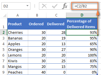
And now, let's see how you can use the Excel percentage formula on real-life data. Suppose, you have the number of "Ordered items" in column B and "Delivered items" in column C. To find out the percentage of delivered products, perform the following steps:
- Enter the formula
=C2/B2in cell D2, and copy it down to as many rows as you need. - Click the Percent Style button (Home tab > Number group) to display the resulting decimal fractions as percentages.
- Remember to increase the number of decimal places if needed, as explained in Percentage tips.
- Done! : )
The same sequence of steps shall be performed when using any other percentage formula in Excel.
In the following example, column D displays a rounded percent of delivered items, without any decimal places showing.
Calculating percentage of total in Excel
In fact, the above example is a particular case of calculating percentages of a total. Now, let's investigate a few more examples that will help you make quick work of calculating a percent of a total in Excel on different data sets.
Example 1. The total is at the end of the table in a certain cell
A very common scenario is when you have a total in a single cell at the end of a table. In this case, the percentage formula will be similar to the one we've just discussed with the only difference that a cell reference in the denominator is an absolute reference (with $).The dollar sign fixes the reference to a given cell, so that it never changes no matter where the formula is copied.
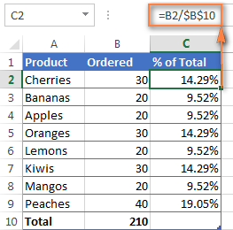
For example, if you have some values in column B and their total in cell B10, you'd use the following formula to calculate percentages of the total:
=B2/$B$10
You use a relative cell reference to cell B2 because you want it to get changed when you copy the formula to other cells of column B. But you enter $B$10 as an absolute cell reference because you want to leave the denominator fixed on B10 when auto-filling the formula down to row 9.
Tip. To make the denominator an absolute reference, either type the dollar sign ($) manually or click the cell reference in the formula bar and press F4.
The screenshot below demonstrates the results returned by the formula, the Percentages of Total column is formatted as percentage with 2 decimal places showing.
Example 2. Parts of the total are in multiple rows
In the above example, suppose you have several rows for the same product and you want to know what part of the total is made by all orders of that particular product.
In this case, you can use the SUMIF function to add up all numbers relating to a given product first, and then divide that number by the total, like this:
=SUMIF(range, criteria, sum_range) / total
Given that column A contains all product names, column B lists corresponding quantities, cell E1 is the name of the product you are interested in, and the total is in cell B10, your real-life formula may look similar to this:
=SUMIF(A2:A9 ,E1, B2:B9) / $B$10
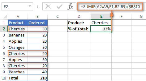
Naturally, you can put the product name directly in the formula, like this:
=SUMIF(A2:A9, "cherries", B2:B9) / $B$10
If you want to find out what part of the total a few different products make, add up the results returned by several SUMIF functions, and then divide that number by the total. For example, the following formula calculates the percent of cherries and apples:
=(SUMIF(A2:A9, "cherries", B2:B9) + SUMIF(A2:A9, "apples", B2:B9)) / $B$10
For more information about the SUM function, please check out the following tutorials:
How to calculate percent difference in Excel
Of all formulas for calculating percentage in Excel, a percent change formula is probably the one you would use most often.
Excel formula for percent increase / decrease
To calculate the percentage of difference between two values A and B, the generic formula is:
When applying this formula to real data, it is important that you correctly determine which value is A and which is B. For example, yesterday you had 80 apples and how you have 100, meaning that now you have 20 apples more than before, which is 25% increase. If you had 100 apples and now you have 80, your number of apples has reduced by 20, which is 20% decrease.
Considering the above, our Excel formula for percentage change takes the following shape:
And now, let's see how you can use this formula for calculating percent difference in your spreadsheets.
Example 1. Calculating percent difference between 2 columns
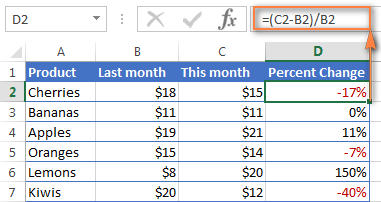
Suppose you have the last month prices in column B and this month prices in column C. Then your percent change formula takes this form:
=(C2-B2)/B2
To calculate the percent difference between two numbers correctly, carry out these steps.
- Enter the formula in any blank cell in row 2, say D2. This will output the result as a decimal number.
- Select the formula cell and click the Percent Style button on the Home tab to convert the decimal number to percentage.
- Drag the formula down to copy it to the below cells.
As the result, the formula calculates the percentage of change in this month (column C) comparted to last month (column B). Positive percentages that show percentage increase are formatted in usual black, while negative percentages (percent decrease) are formatted in red. To have this done automatically, set up a custom format for negative percentages as explained in this tip.
Example 2. Calculating percentage difference between two numbers
In case you have one column of numbers, say column C that lists weekly or monthly sales, you can calculate the percentage change between the previous week/month and the current one using this formula:
=(C3-C2)/C2
Where C2 and C3 are the numbers you are comparing.
Note. Please pay attention that you should skip the first row with data and put your percent difference formula in the 2nd cell, which is D3 in this example.
To display decimals as percentages, apply the percent format to the cells containing your formula, and you will get the following result:
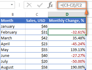
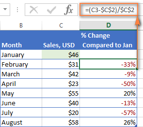
To calculate the percentage of change between a certain number and all other numbers, fix the address of that cell by using the $ sign, e.g. $C$2.
For instance, to calculates the percent increase / decrease for each month compared to January (C2), the formula in D3 is:
=(C3-$C$2)/$C$2
When copying the formula to the below cells, the absolute reference ($C$2) will remain the same, while the relative reference (C3) will change to C4, C5, and so on based on a relative position of the row where the formula is copied.
For more formula examples, please see How to calculate percentage change in Excel.
Calculating amount and total by percentage
As you've just seen, calculating percentages in Excel is easy, and so is calculating amounts and totals if you know the percentage.
Example 1. Calculate amount by total and percentage
Suppose you are buying a new laptop for $950 and they charge 11% VAT on this purchase. The question is - how much do you have to pay on top of the net price? In other words, what is 11% of $950?
The following formula will help:
Assuming that the total value is in cell A2 and percent in B2, the above formula turns into a simple =A2*B2 and returns 104.50.
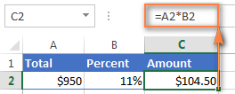
Remember, when you type a number followed by the percent sign (%) in Excel, the number is interpreted as a hundredth of its value. For example, 11% is actually stored as 0.11 and Excel uses this underlying value in all formulas and calculations.
In other words, the formula =A2*11% is equivalent to =A2*0.11. Naturally, you are free to use the decimal number corresponding to the percentage directly in a formula if this works better for your worksheets.
Example 2. Calculating total by amount and percentage
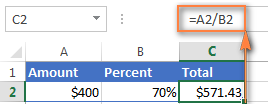
For example, you friend offered you his old computer for $400, which is 30% off the original price. You want to know what the original price was.
Since 30% is the discount, you deduct it from 100% first to know what percentage you actually have to pay (100% - 30% = 70%). Now you need the formula to calculate the original price, i.e. to find the number whose 70% equals 400.
The formula goes as follows:
Applied to real data, it may take any of the following shapes:
=A2/B2
or
=A2/0.7
or
=A2/70%
Tip. To get an answer to a more difficult question - how to calculate the interest amount of a loan payment knowing an interest rate - check out the IPMT function.
How to increase / decrease a number by percentage
The holiday season is upon us and this indicates a change in your usual weekly spendings. You may want to consider different options to find out your optimum weekly allowance.
To increase an amount by a percentage, use this formula:
For example, to increase the value in cell A1 by 20%, the formula is:
=A1*(1+20%)
To decrease an amount by a percentage:
For instance, to reduce the value in cell A1 by 20%, the formula is:
=A1*(1-20%)
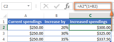
In our example, if A2 is your current expenditures and B2 is the percentage you want to increase or reduce that amount by, here are the formulas you'd enter in cell C2:
Increase by percentage:
=A2*(1+B2)
Reduce by percentage:
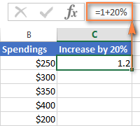
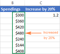
Suppose, you have a column of numbers that you want to increase or reduce by a certain percent, and you want to have the updated numbers in the same column rather than add a new column with the formula. Here are 5 quick steps to handle this task: Increase by percentage: Reduce by percentage: Naturally, you are free to replace 20% in the above formulas with the percentage you want. And here's the result - all the numbers in column B are increased by 20%:
In the same fashion, you can multiply or divide a column of numbers by a certain percentage. Simply enter the desired percentage in an empty cell and follow the steps above.=A2*(1-B2)
How to increase / reduce an entire column by a percentage
=1+20%=1-20%
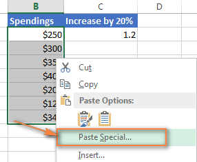
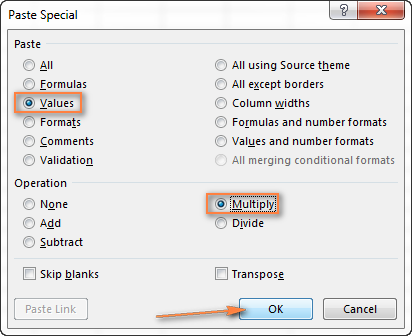
This is how you calculate percentage in Excel. And even if working with percentages has never been your favorite kind of math, by using these basic percentage formulas you can get Excel to do the work for you. That's all for today, thank you for reading!
 by
by
719 comments
I don't even know if this is possible, but I'm trying to make a faster way calculate a customer's price.
In one column I have the retail price, in an adjacent column is where I want to populate the customers price
[$100][ ]
is it possible to have a formula where I just type in the blank column -10%
[$100][-10%]
and through whatever formula it populates as the indented discount
[$100][$90]
would this be possible? the way I'm using excel is as if it's a diary where I'm limited by the space of what's on screen. and I'm trying to keep the number of columns to what's viewed on screen without having to scroll across
Hi! If you have written -10% in a cell, you cannot use Excel to perform calculations in that cell. To calculate percentage, use the recommendations from the article above. Or use VBA.
Hi, I am a teacher at an institution with a new set of students every month, with tests at the end of each month. There are 8 individual tests they need to take up on examination day. I would like to get a running total as well as a running percentage value based on the tests that they have taken thus far. I need this running update so that I can identify the abjectly poorer ones midway and prevent them from taking up the later set of tests if I know they will not meet the pass criteria.
For example, lets say test 1 is for 10 marks, test 2 for 20, test 3 for 30, test 4 for 40, and then repeat till we get 8 tests, amounting to a total of 200 marks.
Lets say the students have taken up 2 tests so far, I would like to obtain the total and relative total percentage value of the tests taken up till now. So I would like to know their total out of 30, as well as their percentage out of 30.
And if I enter the results for test 3, it should automatically show me their totals out of 60, as well as their percentages out of 60.
And once they take up test 4, it should automatically calculate for 100, so on and so forth till all 8 tests are done.
For reference, each test is written in a new column from A-->H, and each student occupies a new row 1-->infinity.
I hope to receive a positive reply that solves my problem. Looking forward to it eagerly.
Thank you!
Hi! If I understand your task correctly, try the following formula:
=SUM(A1:H1)/CHOOSE(COUNT(A1:H1),10,30,60,100,110,130,160,200)
The COUNT function can be used to determine the number of tests completed. CHOOSE function can be used to return the number of marks for any given number of tests. Find the sum of the scores for the completed tests using the SUM function and divide by the number of scores for those tests.
Set the cell with the formula to a percentage number format.
I need formula for percentage rent calculations for gross sales.
Base rent plus percentage of sales with breakpoints.
Sales $0-$800,000.00 pay 7%
Sales 800,000.01-1,300,000.00 pay 3%
Sales 1,300,000.01 - infinity pay 1.5%
Sales were 934,000, they should pay 7% on first 800,000 and pay 3% on the $134,000 additional. I need this formula for my spreadsheet for all months. Helpppppp
Hi! If I understand your task correctly, try to use nested IF formula:
=IF(A1<=800000, A1*0.07, IF(A1<=1300000, (800000*0.07) + ((A1-800000)*0.03), (800000*0.07) + ((1300000-800000)*0.03) + ((A1-1300000)*0.015)))
A1 represents the cell containing the total sales amount (934000 in your example).
The formula uses nested IF statements to check which tier the sales fall into:
Tier 1 (7%): If the sales (A1) are less than or equal to 800000, it simply multiplies the sales by 7% (0.07).
Tier 2 (3%): If the sales (A1) are greater than 800000 but less than or equal to 1300000, it calculates the rent in two parts:
Rent on the first 800000: 800000 * 7%
Rent on the exceeding amount (sales - 800000) at 3%.
Tier 3 (1.5%): If the sales (A1) exceed 1300000, it calculates the rent in three parts:
Rent on the first 800000: 800000 * 7%
Rent on the second tier (1300000 - 800000) at 3%
Rent on the exceeding amount (sales - 1300000) at 1.5%.
Hi, trying to find a formula for percentage of meeting a time of 7 minutes or less.
Hi! I am not sure I fully understand what you mean.
Hello...
I have 30,000 rows of data and 3 columns (Actual premium, Risk premium, Commission). The Actual premiums per row are not the same - they are all different individuals. The Risk premium is a percentage of the Actual premium and the Commission is a percentage of the Actual premium. The Risk % and the Commission % together must be 100% based on the Actual premium amount.
I have to add a formula that calculates each row with the % showing in the Risk and the Commission columns per row for that individual.
Then I have to add a formula in a single empty cell at the top of the Risk premium column and one at the top of the Commission column. These two formulas must be able to change the whole column of Risk % and the same with the Commission %. In other words, If the Risk premium is 90% and the Commission 10% I must be able to only type 90 in the Risk formula cell and 10 in the Commission formula cell for the formula to automatically update all 30 000 rows with different percentages derived from the Actual premium column per row of individual data.
How will I manage to do that? If you can assist I will sincerely appreciate it. Must hand in this spreadsheet by tomorrow and I am struggling now for days on end without success! Hope my explanation is understandable.
Hi! To use the Risk % value in all formulas in column B, write it in cell B1 and use an absolute reference to that cell in the formulas in column B.
Try to enter the following formula in cell B2 and then copy it down along the column: =A2*$B$1
If I understand your task correctly, this article may be helpful: Relative and absolute cell reference: why use $ in Excel formula
Thank you for your reply. Appreciated! Will try it out.
Your formulas don't work in excel. I've tried all of them to calculate the percentage of cell a1 / a1 + b1 in cell c1 and it doesn't work!!!
Hi! I can't guess what data you used and what result you wanted to get. However, if you read the article above carefully, you will see that your formula is not a percentage formula. Perhaps: a1 / (a1 + b1)
Hi! How do I calculate the percent remaining on an invoice log? For example, in cell B3 is my total budget amount. Invoice amounts are listed in column C (C7 - C28). I want to calculate the percentage remaining of my total budget after paying each invoice using column F (F7 - F28). Also, I am tracking the running balance in cell D3 [using the formula =B3 - SUM(C7:C28)]. Any suggestions you can provide are much appreciated!
Hi! All the information you need on how to calculate percentages is in any mathematics textbook, as well as in the article above. Divide D3 by B3.
If I have a desired sales target, ie a number and I have a target % for the Close Rate ratio how would I work out the total number of enquiry required to achieve the sales target. Sales Target 6, Close Rate of 15% means an Enquiry number of ??
Hi! Unfortunately, this information is not enough to understand what you need. You may find the Excel Solver tool useful. Or explain the problem in more detail.
Hi
I hope you can assist. When doing mark ups such as 200% it will be =(D5*2) or 210% will be =(D5*2,1) so is 215% =(D5*2,15)?
Thanks
Having this data on a column, much longer than this, they are ages for 700 employees, what formular will help if i have to determine what % of employee's age is 20years and lesser, 30years and lesser, 4oyears and lesser etc
31 Years, 10 Months, 27 Days
32 Years, 0 Months, 12 Days
123 Years, 5 Months, 16 Days
31 Years, 11 Months, 18 Days
36 Years, 8 Months, 13 Days
30 Years, 4 Months, 14 Days
32 Years, 1 Months, 5 Days
29 Years, 3 Months, 8 Days
29 Years, 7 Months, 4 Days
31 Years, 6 Months, 19 Days
30 Years, 4 Months, 12 Days
39 Years, 2 Months, 4 Days
28 Years, 5 Months, 24 Days
28 Years, 11 Months, 26 Days
26 Years, 9 Months, 8 Days
33 Years, 5 Months, 22 Days
32 Years, 6 Months, 0 Days
38 Years, 2 Months, 16 Days
Hi! If your source data is text, then use a space as a separator and split each value into separate cells. Then use the COUNTIFS function to count the number of values for each condition. Here is the articles that may be helpful to you: How to split cells in Excel: Text to Columns, Flash Fill and formulas, TEXTSPLIT function in Excel: split text strings by delimiter, Count numbers between X and Y using COUNTIFS.
Hi I really hope someone can help.
I want to calculate that out of 1050 is the total and need to know how many tasks i have done this week and last week and then know how much is left in procentage.
Example:
Last week 500 task out of 1050 is complete
This week 670 tasks out of 1050 is complete.
Then i need to know how much in % is left before i reach the goal of 1050
If this could be used in a way for a dynamic diagram, that would be great.
I hope someone can help
i've tried reading the article but i cant figure out which one to use.
Hi! You can count the number of tasks per week using the COUNTIF function. Read more here: Using Excel COUNTIF function with dates.
Hi,
I need your help, I want to calculate % for the following, April Month Traffic is: 55340, and May Month Traffic is 51342, I want to get the result, May Month Traffic is How much % higher or less than the April month traffic. Please help me.
Hi! Pay attention to the following paragraph of the article above: Calculating percent difference between two numbers.
It covers your case completely.
Hi, I need your help, please.
I have 22 trucks in total, and I have their total downtime(time they are not in use) now I meed to get the percentage of the total downtime per week and per month. I hope you can help, below is my example
Truck #1 = 2 days downtime last week (how can I get the percentage of this per week)
Truck #2 = 4 days downtime
Truck #3 = 6 days downtime
Total downtime of 3 trucks last week is 11 (how can I get the percentage of this)
Thanks!
I hope you have studied the recommendations in the tutorial above. It contains answers to your question
=2/12 and percentage format
Weight 20 Score 20
Exp: Weigh Score
WIR/MIR Rejection Rate % 20 20
100 - 95 EXCELLENT
94.9 - 90 VERY GOOD
89.9 - 85 AVERAGE
84.9 - 80 BELOW AVERAGE
79.9 POOR
Please weigh and score make it 100 percentage , PLease help me out this
I’m sorry but your description doesn’t give me a complete understanding of your task. I assume that for your task will be useful Classic nested IF formula.
This article is good.
I am n educator. I have a list of (raw) scores eg. 5, 3, 7, 1, 9. The possible total is 10.
I need a formula that will calculate
1) The percentage of each score
2) The number of scores that are LESS than 40%
I've managed to find a formula that will show how many scores are below 4, but I need to find a way to first calculate the percentage without having to insert an separate column for the percentage.
=COUNTIF(C2:C8,"<4")
Thank you
Hi!
To calculate the percentage, divide by the number of all scores. Please read the above article carefully.
=COUNTIF(C2:C8,"<4")/COUNT(C2:C8)
I have an excel sheet with list of students, theirs' gender, nationalities, seniorities. I have been asked to provide info on breakdown of participants by gender (in %), breakdown of participants by nationalities, breakdown of participants by seniority. I have 2 questions. 1) What does it mean in excel to provide on aforementioned breakdown ? 2) Is there any formula how to do this ? If this is simply calculating percentage, it should be easy, just filtering how many males and females and similar are in the list and then doing count and percentage, but then I am just wondering if i understood correctly what I need to do and whether there is some faster way to do answer problem's questions.
Hi!
To calculate the count by condition, use the COUNTIF function. Then calculate the percentage as described in the article above. I hope I understood the problem correctly.
Hi,
I'm trying to calculate in a chart what percentage of leases expire in each year in one column, 2023, 2024, etc. from a column of varying dates i.e. 1/31/2023, 9/30/2023, 6/30/2024 and also what percentage of square feet of the total building will be represented by the maturing leases each year. What formulas should I use?
Example of output:
Year % Maturing % of Building
2023 40% 25%
2024 10% 5%
Thank you in advance for any help,
JMJ
Hi!
I can't make a chart for you. The calculation of the percentages is described in detail in the article above.
Hello,
I am looking to get a work load / utilization percentage formula depending how many tasks certain employees are assigned to. I have a list of names of all the employees in column M (drop down menu). I am looking to find, how many times they come up within that column and what percent of utilization they are at depending on how many assignments there are assigned to and display that in column P.
Hi!
You can count the number of tasks of each employee using the COUNIF function. There is not enough information to answer your other questions.
Hello, I am looking to get the percentage of a product(s) that was allocated to specific companies in a range of weeks, and then comparing to other range of weeks to know which products in difference were allocated. I have my worksheet set up in the following manner:
The Product and Companies are in Columns (each Company has its respective product) and in the rows I have the weeks and value allocated to each. I need to find the % certain products were allocated.
I hope I was able to explain it. Thank you for your help.
Hello!
To find the percentage, you must first find the amount for the company. To do this, you can use this guide: Excel SUMIFS and SUMIF with multiple criteria.
Hello. I am making a simple spreadsheet to enable me to quote customers. I have it laid out as follows:
In column A: Column B will hold the variable information, eg:
A1: Quantity B1: 1.000
A2: Our buying price B2: 110.00
A3: Margin (in %) B3: 81.82%
A4: Our selling price B4: 200.00
A5: Margin (£'s) B5: £90.00
I have set this up so that B3 is automatically calculated based on the contents of B2 and B4. That is: B3=(B4-B2)/B2*100
I am having to put the selling price in first, in order to calculate the margin percentage.
However! I would also like to be able to enter the margin percentage (B3) first, and have it generate my selling price (B4), based on cost price (B2). But I can't figure out how to do this.
In other words, I would like it to perform both operations: Allow me to manually enter our selling price, and automatically show me margin %, and vice versa - allow me to manually enter a margin %, and automatically show me the selling price.
Is this something anybody can help with?
Thanks in advance!
Hi!
You cannot perform these two operations at the same time using the usual Excel tools, since you cannot write a value and a formula in a cell at the same time. Your task can be accomplished with a VBA macro.
Hi, looking for help attempting to calculate % total from two filters (texts) I am using within my column.
It's for my work to know how many colleagues are using annual leave and flexi days combined.
Along top Row of my excel is Monday to Sunday and columns the name of colleagues.
I want to know at the bottom of the Columns how many people are on Annual Leave and Flexi days using a % for that day of total workforce.
My filters contain start times, finish times, Annual Leave, Flexi and Finish Times etc.
Thanks
Derrick
Hello!
To count the number of values by multiple criteria, use the COUNTIFS function. Here is the article that may be helpful to you: How to use Excel COUNTIFS and COUNTIF with multiple criteria.
I hope I answered your question. If you have any other questions, please don’t hesitate to ask.
Hello, I have two rows, one row says 10, 20, 30, 50, 100, which represent deposit amounts. Below this row shows percentage of the deposits made by customer: for ex. particular customer deposited 5 times, 3 out of which was 10$, so he places 10$ most frequently. Now I want a formula to give me number with the highest percentage below. I mean the formula which will give me number 10. I hope I managed to explain.
Hello!
If I understand your task correctly, find the maximum number using the MAX function. Find the position of this number and extract the corresponding value with INDEX MATCH functions.
=INDEX(A1:E1,MATCH(MAX(A2:E2),A2:E2,0))
I hope my advice will help you solve your task.
Thank u very much.
Hi, if I have 10 columns of numbers together with 1 column indicating the total number of the 10 added up, is there a faster way to find the percentage of each over the total sum? Hope to get help as I have many % to be counted over the total sum.. Thank you.
Hello!
If you need to divide many cells by the same number, then use these recommendations: How to copy formula without changing references. Hope this is what you need.
Hi, I would like to build an excel for different pourcentages applied to a different range of value:
If 0 to 55000 apply 0.5%
55,000.01 to 25000 apply 1%
250,000.01 to 400000 apply 1.5%
400,000.01 to $2,000,000.00 apply 2%
if over $2,000,000: apply 2.5%
How can i do that properly?
Thank you!
Hi!
You can find the answer to your question in the first paragraph of this article - Excel Nested IF statements - examples, best practices and alternatives.
Hi thank you very much, i tried this reading the article but it doesn't return the right pourcentage. =IF((B4=55000.01, B4=250001, B4=400001, B42000000), "")))) do you know why?
Found the solution thank you !
=IF((B4=55000.01, B4=250001, B4=400001, B42000000), ""))))
I need my excel sheet to average a set of numbers as follows: the percent of numbers at or above 70 in a single column.
For example: If my numbers in the column are- 100, 70, 20, 50, 85, 65...what is the percentage of numbers at or above 70.
I know how to calculate this by hand, but is there a way for excel to calculate this?
Hello!
You can determine the percentage of values less than 70 and greater than 70 using the FREQUENCY formula -
=FREQUENCY(A1:A10,69)/COUNT(A1:A10)
Or use COUNTIF function to count the number of values greater than 70 -
=COUNTIF(A1:A10,">=70")/COUNT(A1:A10)
I hope it’ll be helpful.
HI
I WANT TO NOW THE PERCENTAGE BUT THERE IS SUM CONDITIONS. 1, IF THERE IS DATE ITS MEAN WORK DONE. 2 IF THE CELL IS BLANK ITS MEAN WORK TO BE DONE . IF THE CELL HAS "NA" MEAN NO PERCENTAGE REQUIRED.
CELL A1 CELL B1 CELL C1 CELL D1
22.2.22 22.2.22 22.2.22 100% (RESULT SHOULD BE) D1/3
" " NA 22.2.22 50% (RESULT SHOULD BE) D1/2 BECAUSE NA REMOVE IN PERCENTAGE PART
" " " " 22.2.22 33.33% (RESULT SHOULD BE) D1/3 BECAUSE WORK DONE IS 1/3
NA NA NA 0.00% (RESULT SHOULD BE 0 BECAUSE NA IS EXEMPTED IN PERCENTAGE
Hi!
I have a column (Column A) with current year's sales per month and total.
In Column B I have calculated the % of sales attributed to each month (giving a total of 100%).
In Column C I want to calculate the value amount of sales for next target year (I have the overall target for the year) based on the same % per month as current year.
e.g. (Column A) Jan 2021 Sales = 2055 (cell A1); Feb 2021 Sales = 1908 (cell A2) etc giving a total for 2021 of 21619 (cell A13)
(Column B) (rounded to 0 decimal place %) Jan = 10% (cell B1); Feb = 9% (cell B2) etc
(Column C) The overall target total is 24200 (cell C13). What formula to use to get Jan 2022, i.e. 10% of 24200 and Feb 2022, i.e. 9% of 24200
Thanks
Hi!
Pay attention to the following paragraph of the article above – Calculating amount and total by percentage.
=B1*$C$13
Try to enter the following formula in cell C1 and then copy it down along the column. Use an absolute reference to the target total cell.
Thank you so much - I had an incorrect (historic) number format in my destination cells. Your explanation was excellent and worked wonderfully. Thank you again!
Question is:
Condition - order should be supllied within 48 hours (2 days)
Need to calculate the percentage for the amount of orders supllied within 48 hours to see if I am keeping the markup of 90%. Can I know what is the formula to get the calculations between the ordered date and date received with the number of orders.
Hi!
If you have a column in which the supllied time is calculated, then using the SUMIF function, you can calculate the sum of orders completed in 2 hours.
Hi!
I need to find the percentage that $435 is in $2500 but my assessment states that I need to use an Excel formula. What formula do I use?
Hi!
Please re-check the article above since it covers your case.
Hi! Is there a way or a formula of highlighting the values using conditional formatting per say less than 10% of the total without having to calculate the percentages beforehand and a separate row or a column for percentage?
Hi!
The following tutorial should help: Excel formulas for conditional formatting based on another cell value.
Here is an example formula:
=D2/SUM($D$2:$D$10)<0.1
I hope my advice will help you solve your task.
I am trying to find the % of present attendance I have the names going down and the months across. I put an X if they are present at a meeting. At the end I have the total number of meetings they were present at. I need the formula to give me the % of meetings they were present at. so if total is 7 meetings present (column N12) how do I get the % of 7 meetings our of 12. Hope this makes since. Not sure if it does!
Hi!
Pay attention to the second paragraph of the article above. It contains answers to your question.
In column one I have one date and in column two I have another date (which is later in time than the date in column one). Column three needs to reads 50% when column one date has been reached and 100% when column two date has been reached. What would be the formula for column three.
Hello!
Use a nested IF function as described in this guide.
=IF(B1<=TODAY(),100%,IF(A1<=TODAY(),50%,""))
Hope this is what you need.
This is perfect thanks! I am adding to this question
C2 D2 E2 F2
Last year's Drill Drill #1 Date Drill #2 forcasted Date Conformance %
5/5/2022 5/30/2022 50.00%
I need to show when we are within 6 months of last years drill dates. D2 has to be within 6 months of C2. When D2 is completed within 6 months of C2 I would like D2 cell to turn green. When D2 date is 30 days out from hitting the size month mark and has not been complete I would like the cell to turn yellow. If the C2 date is equal to or past the D2 date I would like the D2 cell to turn red.
Hello!
The answer to your question can be found in this article: How to conditionally format dates and time in Excel - built-in rules and formulas.
I hope it’ll be helpful.
I got the cell to turn red and the cell read "false" but I could not keep the date in the cell. How would I keep the color in the cell and keep the date?
Hi!
I cannot understand your problem. Create a conditional formatting rule and specify the desired color there.
Column A has a date, column B has a future date from column A. When column A date is a month away from column B date, I need column B cell to show yellow. When column A date matches column B date or go passed column B date I need column B cell to show red.
Hi!
If I understand your task correctly, the following formulas should work for you:
=A1+30 > B1
=A1
Hello,
I am trying to provide a percentage from column B divided by column A giving the resulted percentage of blanks in column B. What would be the formula for this?
Thank you.
Hi!
I am not sure I fully understand what you mean.
Hello!
I have exported a customers account activity to excel. one of the columns is for Drop ship (or DS). This is when we are shipping a product to a third party for our customer instead of shipping it directly to our customer. Every row representing an invoice for this customer either has a DS or is blank in this DS column. how do I calculate the percentage of Drop ships vs. none Drop ships at the bottom??
Hello!
Use the COUNTIF function to count the number of values for a condition.
=COUNTIF(A1:A20,"DS")/COUNTIF(A1:A20,"")
This should solve your task.
Hello, I'm trying to figure out how likely an event might happen given a string of prior events. Let's say player A has been selected in 10 drafts (2 player taken, 3rd, 2nd, 1st, 2nd, 5th, 1st, 3rd, 4th and 1st). I want to know what draft slot would he still be available in 90% of drafts, 75% of drafts, 50%, 25% and 10%. How can I do this in excel? Math is hard, Thanks!
Hi!
If you describe to me the sequence of calculations, I can help you write the formula.
Hello Alexander, thank you for responding. I am not sure of the sequence of calculations, that's what I am hoping to get help with. I am trying to recreate some work I found online by an amazing fantasy baseball writer. He pulled data from several types of leagues, they differ in the types of scoring used to the amount of teams in the league. I am only pulling the data that most resembles the league I play in. From the data he was able to determine what pick players might be drafted in future drafts. For instance in 90% of drafts such and such player would still be available pick 3, in 75% of drafts they might still be available pick 5 and so on. I tried to use the PROB function but I wasn't sure how to set it up. I kept getting the #N/A error. Is this enough information to help?
Hi, I have a list of products that are different days old (manufactured on different stages)
I want to calculate out of this list what percentage of the products are between10 and 20 days old, 20 and 30days old etc. What formula can I use?
For instance:
Product 1 - 10 days
Product 2 - 11 days
Product 3 - 12 days
Product 4 - 20 days
Product 5 - 22 days
Product 6 - 31 days
Would I be able to use a formula to calculate the % of products between 10 - 20days and 20 - 30 days etc.
Easy enough if sitting with say 6 products but not so easy if 1000's of products.
Thanks!
Hello!
The formula below will do the trick for you:
=FREQUENCY(A1:A10,D1:D4)/COUNT(A1:A10)
A1:A10 - your data (days)
D1:D4 - grouping value range (9, 19, 29,39)
Set formula cells to percentage format.
hello sir, i want to ask you something. if i have value like 50 how much it will be 100%. what formula do i need for this one?
Hi, Can you help me calculate a running/cumulative percentage? Meaning if I took a price increase of 4% in April, a 6% price increase in June, 0% price increase in November and a 7% price increase in December. How can I calculate the total % of the increase in a year? I cannot just total them up. But I don't know how to create the formula that builds them up to the correct %. I'd like to create the formula for a 12 month period, where some months took 0% for certain products.
Thanks
Hello!
If you have 12 months, then in this case you can use the formula for calculating the average.
=SUM(A1:A12)/12
If the weight of each value is not the same, use the weighted average calculation.
Good job,pease I have an inventory stock project,please help me out on ho to calculate 30%, here is the sample ( goods is sold at 450 in cell A, now how do I subtract 30% from 450 in Xcel thanks
Hi!
Pay attention to the following paragraph of the article above - How to increase / decrease a number by percentage.
Hello,
I have a series of numbers.
D2 = 50
D6 = 5
E2 = 25
E6 = 10
F2 = 32
F6 = 15
first I am doing this =sum(D6*D2)+(E2*E6)+(F2*F6)
Now, I need to subtract 18% of E6 before I can multiply E2*E6
I have tried numerous way with no success. Like: =sum(D6*D2)+((E2-18%)*E6)+(F2*F6)
Can you help?
Hi!
Please try the following formula:
=D6*D2+E2*E6*(1-0.18)+F2*F6
help needed!!
what formula do I use if to work out the percentage of complaints per 100,000 customers
info
week 1 - 655235 customers with 45 complaints
week 2 - 698465 customers with 48 complaints
and so on and so on......
thank you in advance
Hi!
Please re-check the article above since it covers your task.
=B1/A1*100%
I am trying to come up with a formula for positive time stats. I’ve downloaded the report from Cognos that breaks down each time status used in the system and I I want to be able to convert specific cells “stats” minutes into percentages of total minutes worked. I want to use this to help with time management. Any ideas?
Using simple formula for positive time stat: active minutes (450) /total minutes worked (510) *100
Hi!
I don't know how you define active minutes. But I think that you can use the SUMIF function to count active minutes. I can't give you more specific advice because I don't have more information from you.
I have total costs of each individual job task for a single Purchase Order Value for work to be performed. I have to charge 10.2% tax total for the entire job but need to show breakdown of tax per individual job task. All of my totals in Row 6 have to be taxed at 10.2% in equal increments. Not all scenarios will have require all job tasks so I would also need to exclude any costs of $0. TIA
Hello!
You can get a list of tasks for an individual job that has a cost greater than 0 using the FILTER function. For detailed instructions, see this article: Filter with multiple AND criteria.
I hope it’ll be helpful. If something is still unclear, please feel free to ask.