The tutorial explains how to use the nested IF function in Excel to check multiple conditions. You will also learn a few other functions that could be good alternatives to using a nested formula in Excel.
How do you usually implement a decision-making logic in your Excel worksheets? In most cases, you'd use an IF formula to test your condition and return one value if the condition is met, another value if the condition is not met. To evaluate more than one condition and return different values depending on the results, you nest multiple IFs inside each other.
Though very popular, the nested IF statement is not the only way to check multiple conditions in Excel. In this tutorial, you will find a handful of alternatives that are definitely worth exploring.
Excel nested IF statement
Here's the classic Excel nested IF formula in a generic form:
You can see that each subsequent IF function is embedded into the value_if_false argument of the previous function. Each IF function is enclosed in its own set of parentheses, but all the closing parentheses are at the end of the formula.
Our generic nested IF formula evaluates 3 conditions, and returns 4 different results (result 4 is returned if none of the conditions is TRUE). Translated into a human language, this nested IF statement tells Excel to do the following:
test condition2, if TRUE - return result2, if FALSE -
test condition3, if TRUE - return result3, if FALSE -
return result4
As an example, let's find out commissions for a number of sellers based on the amount of sales they've made:
| Commission | Sales |
| 3% | $1 - $50 |
| 5% | $51 - $100 |
| 7% | $101 - $150 |
| 10% | Over $150 |
In math, changing the order of addends does not change the sum. In Excel, changing the order of IF functions changes the result. Why? Because a nested IF formula returns a value corresponding to the first TRUE condition. Therefore, in your nested IF statements, it's very important to arrange the conditions in the right direction - high to low or low to high, depending on your formula's logic. In our case, we check the "highest" condition first, then the "second highest", and so on:
=IF(B2>150, 10%, IF(B2>=101, 7%, IF(B2>=51, 5%, IF(B2>=1, 3%, ""))))
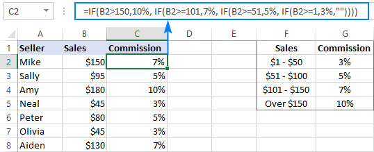
If we placed the conditions in the reverse order, from the bottom up, the results would be all wrong because our formula would stop after the first logical test (B2>=1) for any value greater than 1. Let's say, we have $100 in sales - it is greater than 1, so the formula would not check other conditions and return 3% as the result.
If you'd rather arrange the conditions from low to high, then use the "less than" operator and evaluate the "lowest" condition first, then the "second lowest", and so on:
=IF($B2<1, 0%, IF($B2<51, 3%, IF($B2<101, 5%, IF($B2<=150, 7%, 10%))))
As you see, it takes quite a lot of thought to build the logic of a nested IF statement correctly all the way to the end. And although Microsoft Excel allows nesting up to 64 IF functions in one formula, it is not something you'd really want to do in your worksheets. So, if you (or someone else) are gazing at your Excel nested IF formula trying to figure out what it actually does, it's time to reconsider your strategy and probably choose another tool in your arsenal.
For more information, please see Excel nested IF statement.
Nested IF with OR/AND conditions
In case you need to evaluate a few sets of different conditions, you can express those conditions using OR as well as AND function, nest the functions inside IF statements, and then nest the IF statements into each other.
Nested IF in Excel with OR statements
By using the OR function you can check two or more different conditions in the logical test of each IF function and return TRUE if any (at least one) of the OR arguments evaluates to TRUE. To see how it actually works, please consider the following example.
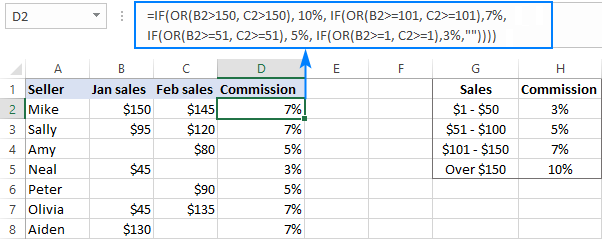
Supposing, you have two columns of sales, say January sales in column B and February sales in column C. You wish to check the numbers in both columns and calculate the commission based on a higher number. In other words, you build a formula with the following logic: if either Jan or Feb sales are greater than $150, the seller gets 10% commission, if Jan or Feb sales are greater than or equal to $101, the seller gets 7% commission, and so on.
To have it done, write a few OF statements like OR(B2>150, C2>150) and nest them into the logical tests of the IF functions discussed above. As the result, you get this formula:
=IF(OR(B2>150, C2>150), 10%, IF(OR(B2>=101, C2>=101),7%, IF(OR(B2>=51, C2>=51), 5%, IF(OR(B2>=1, C2>=1), 3%, ""))))
And have the commission assigned based on the higher sales amount:
For more formula examples, please see Excel IF OR statement.
Nested IF in Excel with AND statements
If your logical tests include multiple conditions, and all of those conditions should evaluate to TRUE, express them by using the AND function.
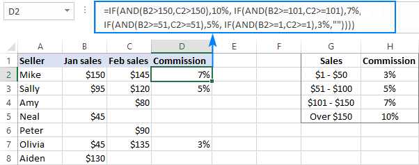
For example, to assign the commissions based on a lower number of sales, take the above formula and replace OR with AND statements. To put it differently, you tell Excel to return 10% only if Jan and Feb sales are greater than $150, 7% if Jan and Feb sales are greater than or equal to $101, and so on.
=IF(AND(B2>150, C2>150), 10%, IF(AND(B2>=101, C2>=101), 7%, IF(AND(B2>=51, C2>=51), 5%, IF(AND(B2>=1, C2>=1), 3%, ""))))
As the result, our nested IF formula calculates the commission based on the lower number in columns B and C. If either column is empty, there is no commission at all because none of the AND conditions is met:
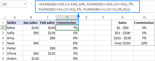
If you'd like to return 0% instead of blank cells, replace an empty string (''") in the last argument with 0%:
=IF(AND(B2>150, C2>150), 10%, IF(AND(B2>=101, C2>=101), 7%, IF(AND(B2>=51, C2>=51), 5%, IF(AND(B2>=1, C2>=1), 3%, 0%))))
More information can be found here: Excel IF with multiple AND/OR conditions.
VLOOKUP instead of nested IF in Excel
When you are dealing with "scales", i.e. continuous ranges of numerical values that together cover the entire range, in most cases you can use the VLOOKUP function instead of nested IFs.
For starters, make a reference table like shown in the screenshot below. And then, build a Vlookup formula with approximate match, i.e. with the range_lookup argument set to TRUE.
Assuming the lookup value is in B2 and the reference table is F2:G5, the formula goes as follows:
=VLOOKUP(B2,$F$2:$G$5,2,TRUE)
Please notice that we fix the table_array with absolute references ($F$2:$G$5) for the formula to copy correctly to other cells:
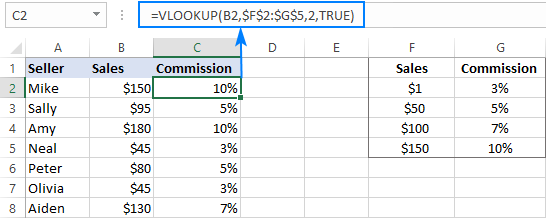
By setting the last argument of your Vlookup formula to TRUE, you tell Excel to search for the closest match - if an exact match is not found, return the next largest value that is smaller than the lookup value. As the result, your formula will match not only the exact values in the lookup table, but also any values that fall in between.
For example, the lookup value in B3 is $95. This number does not exist in the lookup table, and Vlookup with exact match would return an #N/A error in this case. But Vlookup with approximate match continues searching until it finds the nearest value that is less than the lookup value (which is $50 in our example) and returns a value from the second column in the same row (which is 5%).
But what if the lookup value is less than the smallest number in the lookup table or the lookup cell is empty? In this case, a Vlookup formula will return the #N/A error. If it's not what you actually want, nest VLOOKUP inside IFERROR and supply the value to output when the lookup value is not found. For example:
=IFERROR(VLOOKUP(B2, $F$2:$G$5, 2, TRUE), "Outside range")
Important note! For a Vlookup formula with approximate match to work correctly, the first column in the lookup table must be sorted in ascending order, from smallest to largest.
For more information, please see Exact match VLOOKUP vs. approximate match VLOOKUP.
IFS statement as alternative to nested IF function
In Excel 2016 and later versions, Microsoft introduced a special function to evaluate multiple conditions - the IFS function.
An IFS formula can handle up to 127 logical_test/value_if_true pairs, and the first logical test that evaluates to TRUE "wins":
In accordance with the above syntax, our nested IF formula can be reconstructed in this way:
=IFS(B2>150, 10%, B2>=101, 7%, B2>=51, 5%, B2>0, 3%)
Please pay attention that the IFS function returns the #N/A error if none of the specified conditions is met. To avoid this, you can add one more logical_test/value_if_true to the end of your formula that will return 0 or empty string ("") or whatever value you want if none of the previous logical tests is TRUE:
=IFS(B2>150, 10%, B2>=101, 7%, B2>=51, 5%, B2>0, 3%, TRUE, "")
As the result, our formula will return an empty string (blank cell) instead of the #N/A error if a corresponding cell in column B is empty or contains text or negative number.
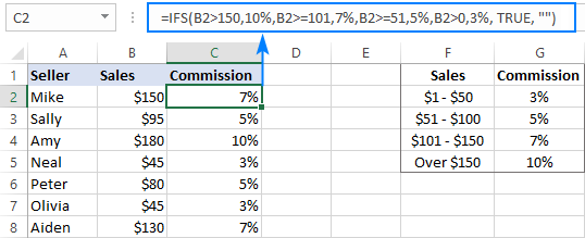
Note. Like nested IF, Excel's IFS function returns a value corresponding to the first condition that evaluates to TRUE, which is why the order of logical tests in an IFS formula matters.
For more information, please see Excel IFS function instead of nested IF.
CHOOSE instead of nested IF formula in Excel
Another way to test multiple conditions within a single formula in Excel is using the CHOOSE function, which is designed to return a value from the list based on a position of that value.
Applied to our sample dataset, the formula takes the following shape:
=CHOOSE((B2>=1) + (B2>=51) + (B2>=101) + (B2>150), 3%, 5%, 7%, 10%)
In the first argument (index_num), you evaluate all the conditions and add up the results. Given that TRUE equates to 1 and FALSE to 0, this way you calculate the position of the value to return.
For example, the value in B2 is $150. For this value, the first 3 conditions are TRUE and the last one (B2 > 150) is FALSE. So, index_num equals to 3, meaning the 3rd value is returned, which is 7%.
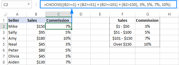
Tip. If none of the logical tests is TRUE, index_num is equal to 0, and the formula returns the #VALUE! error. An easy fix is wrapping CHOOSE in the IFERROR function like this:
=IFERROR(CHOOSE((B2>=1) + (B2>=51) + (B2>=101) + (B2>150), 3%, 5%, 7%, 10%), "")
For more information, please see Excel CHOOSE function with formula examples.
SWITCH function as a concise form of nested IF in Excel
In situations when you are dealing with a fixed set of predefined values, not scales, the SWITCH function can be a compact alternative to complex nested IF statements:
The SWITCH function evaluates expression against a list of values and returns the result corresponding to the first found match.
In case, you'd like to calculate the commission based on the following grades, rather than sales amounts, you could use this compact version of nested IF formula in Excel:
=SWITCH(C2, "A", 10%, "B", 7%, "C", 5%, "D", 3%, "")
Or, you can make a reference table like shown in the screenshot below and use cell references instead of hardcoded values:
=SWITCH(C2, $F$2, $G$2, $F$3, $G$3, $F$4, $G$4, $F$5, $G$5, "")
Please notice that we lock all references except the first one with the $ sign to prevent them from changing when copying the formula to other cells:
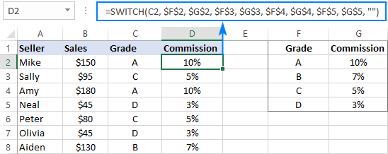
Note. The SWITCH function is only available in Excel 2016 and higher.
For more information, please see SWITCH function - the compact form of nested IF statement.
Concatenating multiple IF functions in Excel
As mentioned in the previous example, the SWITCH function was introduced only in Excel 2016. To handle similar tasks in older Excel versions, you can combine two or more IF statements by using the Concatenate operator (&) or the CONCATENATE function.
For example:
=(IF(C2="a", 10%, "") & IF(C2="b", 7%, "") & IF(C2="c", 5%, "") & IF(C2="d", 3%, ""))*1
Or
=CONCATENATE(IF(C2="a", 10%, ""), IF(C2="b", 7%, ""), IF(C2="c", 5%, "") & IF(C2="d", 3%, ""))*1
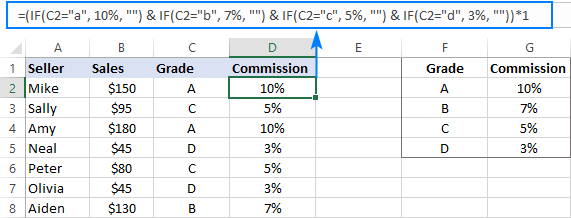
As you may have noticed, we multiply the result by 1 in both formulas. It is done to convert a string returned by the Concatenate formula to a number. If your expected output is text, then the multiplication operation is not needed.
For more information, please see CONCATENATE function in Excel.
You can see that Microsoft Excel provides a handful of good alternatives to nested IF formulas, and hopefully this tutorial has given you some clues on how to leverage them in your worksheets. To have a closer look at the examples discussed in this tutorial, you are welcome to download our sample workbook below. I thank you for reading and hope to see you on our blog next week!
Practice workbook for download
Excel nested If statement - examples (.xlsx file)
 by
by
226 comments
Fyi the IFS function apparently behaves differently than nested IF(IF( ))s. IFS does not stop when it finds a true condition but instead evaluates everything, which can cause slowdowns with large datasets or complicated conditions/formulas when true. Although seemingly archaic, nested IF statements may be the way to go for some (if readability is less of a priority).
I am tracking the mileage from 42 potential combinations of "to" and "from" locations. I have one column of the "from" location (CO, JWE, EL, PA, etc.) and a second column of the "to" location (CO, JWE, EL, PA, etc.). I want to calculate if column 1 says CO and column 2 says BDM then I want column 3 to generate the text "2.1". Here is my formula. What am I doing wrong, or is there a limit to the amount of ifs I can use in one cell?
=IF(AND(D2="CO", E2="PK"), "1.2", IF(AND(D2="CO", E2="JWE"), "1.2", IF(AND(D2="CO", E2="EL"), "2.3", IF(AND(D2="CO", E2="PA"), "2.0", IF(AND(D2="CO", E2="NV"), "1.9", IF(AND(D2="CO", E2="BDM"), "2.1", IF(AND(D2="PK", E2="CO"), "1.2", IF(AND(D2="PK", E2="JWE"), "0.2", IF(AND(D2="PK", E2="EL"), "1.6", IF(AND(D2="PK", E2="PA"), "2.1”, IF(AND(D2="PK", E2="NV"), "0.6", IF(AND(D2="PK", E2="BDM"), "1.4", IF(AND(D2="JWE", E2="CO"), "1.2", IF(AND(D2="JWE", E2="PK"), "0.2", IF(AND(D2="JWE", E2="EL"), "1.6", IF(AND(D2="JWE", E2="PA"), "1.8", IF(AND(D2="JWE", E2="NV"), "1.0", IF(AND(D2="JWE", E2="BDM"), "1.4", IF(AND(D2="EL", E2="CO"), "2.3", IF(AND(D2="EL", E2="PK"), "1.6", IF(AND(D2="EL", E2="JWE"), "1.5", IF(AND(D2="EL", E2="PA"), "1.4", IF(AND(D2="EL", E2="NV"), "0.9", IF(AND(D2="EL", E2="BDM"), "2.4", IF(AND(D2="PA", E2="CO"), "2.0", IF(AND(D2="PA", E2="PK"), "2.1", IF(AND(D2="PA", E2="JWE"), "1.8", IF(AND(D2="PA", E2="EL"), "1.4", IF(AND(D2="PA", E2="NV"), "1.9", IF(AND(D2="PA", E2="BDM"), "3.0", IF(AND(D2="NV", E2="CO"), "1.9", IF(AND(D2="NV", E2="PK"), "0.6", IF(AND(D2="NV", E2="JWE"), "1.0", IF(AND(D2="NV", E2="EL"), "0.9", IF(AND(D2="NV", E2="PA"), "1.9", IF(AND(D2="NV", E2="BDM"), "1.6", IF(AND(D2="BDM", E2="CO"), "2.1", IF(AND(D2="BDM", E2="PK"), "1.4", IF(AND(D2="BDM", E2="JWE"), "1.4", IF(AND(D2="BDM", E2="EL"), "2.4", IF(AND(D2="BDM", E2="PA"), "3.0", IF(AND(D2="BDM", E2="NV"), "1.6"))))))))))))))))))))))))))))))))))))))))))
Hi! You used the wrong quotation marks: "2.1”.
For multiple conditions, I recommend using the IFS formula as described in this article: The new Excel IFS function instead of multiple IF.
Required an alternate formula for below one
IF($A$119<=$A127,$A$119:$E$119,IF($A$118<=$A127,$A$118:$E$118,$A$117:$E$117))
need to reduce the number of time to select the row if the rows shall be more than 100
Sorry, it's not quite clear what you are trying to achieve. Please clarify your specific problem or provide additional information to understand what you need.
In vlookup function in order to choose the specific row in the table based on certain cell condition we are using multiple if condition
If table contains multiple row what is the alternative method
Hi! From what you've described, it's hard to fully understand what you're being asked to do. Maybe this article will be helpful: How to Vlookup multiple values in Excel with criteria.
Hi!
The following nested IF formula is skipping over the third and fourth lines if the second line returns an #N/A. I've tried alternative approaches (i.e., CHOOSE, etc.) which didn't work either. The basic idea is for the cell to display a certain text given the appearance of a cell reference within specific lists which are located on disparate Sheets. For future maintenance, I wish to avoid utilizing VLOOKUP. The data have all been formatted as Text.
=IFNA(IF('FAF Queues'!E2="","",
IF('Queues'!E2=INDEX('State 1 Full'!A:A, MATCH('Queues'!E2, 'State 1 Full'!A:A, 0)), "State 1",
IF('Queues'!E2=INDEX('State 1 Custom'!A:A, MATCH('Queues'!E2, 'State 1 Custom'!A:A, 0)), "Custom",
IF('Queues'!E2=INDEX('State 2 Full'!A:A, MATCH('Queues'!E2, 'State 2 Full'!A:A, 0)), "State 2", "Non Urgent")))),
"Not working")
Is there a way to ensure each nested IF is processed in succession, despite the #N/A being returned? #N/A occurs whether or not I use the IFNA piece of the formula.
Thank you!
Correction to formula to reduce confusion:
=IFNA(IF('Queues'!E2="","",
IF('Queues'!E2=INDEX('State 1 Full'!A:A, MATCH('Queues'!E2, 'State 1 Full'!A:A, 0)), "State 1",
IF('Queues'!E2=INDEX('State 1 Custom'!A:A, MATCH('Queues'!E2, 'State 1 Custom'!A:A, 0)), "Custom",
IF('Queues'!E2=INDEX('State 2 Full'!A:A, MATCH('Queues'!E2, 'State 2 Full'!A:A, 0)), "State 2", "Non Urgent")))),
"Not working")
**NOTE: "Not working" is simply being used to identify the instances of #N/A, and it will be changed if this ends up working.
Hi! To ignore the error message and replace it with a value or formula, use the IFERROR function. You can find the examples and detailed instructions here: How to use IFERROR in Excel with formula examples. I don't have your data, so I can't change your formula.
My question is really: why does this nested IF skip from IF('Queues'!E2=INDEX('State 1 Full'!A:A, MATCH('Queues'!E2, 'State 1 Full'!A:A, 0)), "State 1" to "Not working"? What am I missing?
Shouldn't it move from IF('Queues'!E2=INDEX('State 1 Full'!A:A, MATCH('Queues'!E2, 'State 1 Full'!A:A, 0)), "State 1"
to IF('Queues'!E2=INDEX('State 1 Custom'!A:A, MATCH('Queues'!E2, 'State 1 Custom'!A:A, 0)), "Custom"
then to IF('Queues'!E2=INDEX('State 2 Full'!A:A, MATCH('Queues'!E2, 'State 2 Full'!A:A, 0)), "State 2", "Non Urgent"
before going to "Not working"?
Hi! I already answered you: use the IFERROR or IFNA function.
If INDEX('State 1 Full'!A:A, MATCH(Queues!E1, 'State 1 Full'!A:A, 0)) returns #N/A, then the formula immediately returns #N/A.
Read carefully the article on the IFERROR function I recommended, as well as How to use IFNA function in Excel with examples.
I'm not sure how to do this problem, but I am trying to find the insurance plan rate for a person in a table (exported insurance bill) that has columns for name, insurance plan number (4 levels - 1 is only for executives so not really used), and coverage level. I ADD a column for whether or not the employee is in category A, O or T (but now A&O have the same rates, so would only need if T or not T classification) [ when I have time, I will update our master conversion of employees, but that has yet to arrive].
I need to look up the plan coverage rate for an employee based on their classification (if equals T), then if T find the plan name and coverage level and return the rate or if NOT T, do the same, but for it's own set of rates.
I set up master arrays with coverage level in column A1 (COL HEADING) and variables in A2:A5 (IND, ESC, ECH & FAM)
Plan numbers in column headings for col B-D (A02, A03, A04)
Rates are in grid of B2:D5
all others (not T classified)
CVG_LVL Plan 1 (A02) Plan 2 (A03) Plan 3 (A04)
Employee 90.00 $100.00 $138.00
Employee + Spouse 275.00 $300.00 $350.00
Employee + Child(ren) 250.00 $200.00 $320.00
Employee + Family 450.00 $500.00 $530.00
for T classified
CVG_LVL Plan 1 (A02) Plan 2 (A03) Plan 3 (A04)
Employee 65.00 $71.00 $100.00
Employee + Spouse 230.00 $261.00 $299.00
Employee + Child(ren) 205.00 $233.00 $263.00
Employee + Family 370.00 $423.00 $469.00
I'm stuck. I can get the xlookup to tell me the employee name and return their respective departments and percentages of the rate to code to each department, BUT I can't seem to figure out how to get the rate based on their classification and then given that, use the coverage level to ultimately return the rate for that employee.
Any suggestions is appreciated.
Hello! Unfortunately, I couldn't make sense of the large and complicated description of your data. Try to make it simpler, write source data and desired result.
Use a function or formula to calculate the commission for each truck driver based on this information: (Drivers' commission is a percentage of their Grand Total. Those with 70,000 or less, get a 5% commission. Drivers whose grand total is above 70,000 get a 10% commission.) 3 marks
Study the article above carefully and get your 3 marks.
Hi, I am trying to get my formula to work. The end result would be if a1 > b1 then "apple". if b1> c1 then "orange" and if c1> a1 then " pineapple" however., I seem to get stuck when in the second row. my current formula is =IF(A>B1,"APPLE",IF(B1>A1,"ORANGE",IF(C1>B1,"PINEAPPLE",IF(A1>C1,"APPLE",IF(B1>C1,"ORANGE",IF(C1>A1,"Packout"))))))
Hi! In your case, several conditions can be executed simultaneously. So pay attention to this paragraph: Nested IF with OR/AND conditions. It is impossible to correct your formula, because you have not described these conditions.
Hello and thank you for great content! I'm having problems with my formula. In one cell I have an answer (C33="Yes"). In another cell (B32) I have a number value. The returned value differs based on the number value in cell B32. The formula pulls in the correct value for the very first condition where B32<65%. Every statement after the first one doesn't seem to work. When I enter a value of 65% or greater in B32 it just returns 0. Should I be using a different formula? Thank you for any help you can provide.
=IF(AND(C33="Yes",B32<65%),Values!V4, IF(AND(C33="Yes",65%<B32<75%),Values!V5, IF(AND(C33="Yes",75%<B32<80%),Values!V6, IF(AND(C33="Yes",80%<B32<85%),Values!V7, IF(AND(C33="Yes",85%<B32<90%),Values!V8, IF(AND(C33="Yes",90%<B32<95%),Values!V9,0))))))
Hi! The statement 65%Excel AND function.
Hi Alexander, I didn't refresh my browser so I didn't see your reply until after posting the solution we found. Thank you for taking a look!
I figured it out! Well, actually, my husband did. For anyone reading, the issue was that the B32 range wasn't recognized (i.e. 65%<B32<75%). Using this same example, since the condition for the value up to 65% is already accounted for in the previous condition, only B32<75% needs to be written in the next condition. Still open to simplifications to this formula if any exist. Thanks!
I am trying to write a formula that references a date range based on age that will return a value from a list of values to calculate a certain premium amount.
For example if the person is aged 54.85 then I need to return a value of 0.43 (the table reference is G$28) which is is the age range of 50 and less than 55 - i have written the following formula but it is not working for me at all
=IF(AND(F5=25,F5=29,F5=35,F5=40,F5=45,F5=50,F5=55,F5=60,F5=65,F570,G$32))))
and I have tried it this way
=IF(IF(F4=25,F4=30,F4=35,F4=40,F4=45,F4=50,F4=55,F4=60,F4=65,F470,G$32))))
Hi! Try using the approximate match Vlookup formula to search in value intervals. You can find the examples and detailed instructions here: How to Vlookup for approximate match.
I hope it’ll be helpful. If something is still unclear, please feel free to ask.
Thank you, very well written article
I need some help with a formula
I have the below formula that calculates the sum of money someone would get for allowances for Breakfast, Lunch and Dinner when travelling.
G20, H20, I20 – are separate criteria’s if blank add it if not do not add (you would indicate in these columns if a meal is provided, B, L, D)
The Sheet H, I, J columns are the count column
D20 is a criteria (location) and L7 is a criteria (status)
=IF(G20="",SUM((SUMIFS('SHEET as at 26 May 23'!$H$7:$H$30,'SHEET as at 26 May 23'!$B$7:$B$30,$D20,'SHEET as at 26 May 23'!$D$7:$D$30,$L$7))))+IF(H20="",SUM((SUMIFS('SHEET as at 26 May 23'!$I$7:$I$30,'SHEET as at 26 May 23'!$B$7:$B$30,$D20,'SHEET as at 26 May 23'!$D$7:$D$30,$L$7))))+IF(I20="",SUM((SUMIFS('SHEET as at 26 May 23'!$J$7:$J$30,'SHEET as at 26 May 23'!$B$7:$B$30,$D20,'SHEET as at 26 May 23'!$D$7:$D$30,$L$7))))
What I now need to do is subtract an amount for meals dependent on what time someone departs home or arrives back home I have a column for departure and arrival times
For departure
If depart before 07:00 = above formula
If depart after 07:01 subtract the answer to: SUMIFS('SHEET as at 26 May 23'!$H$7:$H$30,'SHEET as at 26 May 23'!$B$7:$B$30,$D20,'SHEET as at 26 May 23'!$D$7:$D$30,$L$7)
If depart after 13:01 subtract answer to: SUMIFS('SHEET as at 26 May 23'!$H$7:$H$30,'SHEET as at 26 May 23'!$B$7:$B$30,$D20,'SHEET as at 26 May 23'!$D$7:$D$30,$L$7) + SUM((SUMIFS('SHEET as at 26 May 23'!$I$7:$I$30,'SHEET as at 26 May 23'!$B$7:$B$30,$D20,'SHEET as at 26 May 23'!$D$7:$D$30,$L$7)
If depart after 19:01 = answer is zero
For arrival back home
If return prior to 07:00 = answer is zero
If return after 07:01 but before 13:00 answer is SUMIFS('SHEET as at 26 May 23'!$H$7:$H$30,'SHEET as at 26 May 23'!$B$7:$B$30,$D20,'SHEET as at 26 May 23'!$D$7:$D$30,$L$7)
If return after 13:01 but before 19:00 answer is SUMIFS('SHEET as at 26 May 23'!$H$7:$H$30,'SHEET as at 26 May 23'!$B$7:$B$30,$D20,'SHEET as at 26 May 23'!$D$7:$D$30,$L$7) + SUM((SUMIFS('SHEET as at 26 May 23'!$I$7:$I$30,'SHEET as at 26 May 23'!$B$7:$B$30,$D20,'SHEET as at 26 May 23'!$D$7:$D$30,$L$7)
If arrive after 19:01 answer is original formula.
I have played around with IF formulas and time but cant work out how to add formulas instead of an actual number
=IF(E20="","0",IF(E20<TIME(7,0,0),"1",IF(E20<TIME(13,0,1),".75",IF(E20TIME(19,0,1),"0")))))
I have also played around with trying to break it up into separate columns and then adding these columns together which works for another allowance structure although I now have 20 columns in the background with various formulas,
But this allowance structure is not working and I am hoping I can make it tidier
Can you help please???
Hi! It is very difficult to understand a formula that contains unique references to your workbook worksheets. I cannot guess what is not working in your formulas. I have no data to check how these formulas work. Ask me a concrete question about the formula, and I will try to help.
I would like to produce an equation where the range of sales range will produce a dollar amount based on the commission %. The equation in the article is just producing a %.
Example:
0 - $50k apply 4.75%
50.01K to $150k apply 3%
Over $150k apply 1.50%
Based on this scale, if the there were 1,000,000 of sales, the answer would be $18,125, but I can't get the IF formula to work.
Thank you!
Please re-check the article above since it covers your task. See first paragraph.
Hi all,
I am trying to nest a lot of if statements together, some are just "if then", others are "if then else".
I am having difficulty with the syntax.
I can see you can use concatenate to combine multiple "if then else" statements together, but what if I wanted to combine a mix of "if then", "if then", "if then else", "if then else" for example.
I keep getting a "too many arguments" error
The details aren't important, just the syntax.
My example is :
=If(M7="Commencement",1500,IF(M7="Recommencement",750,IF(AND(M7="BAC 1st Qtr",O4*.5>7000),7000,O4*.5,IF(AND(M7="BAC 1st Qtr",O4*.5>4000),4000,O4*.9))))
I appreciate any assistance
Hi! Pay attention to this part of the formula.
IF(AND(M7="BAC 1st Qtr",O4*.5>7000),7000,O4*.5, IF....
This IF has two FALSE arguments.
If you have many IF arguments, I recommend using the IFS function.
Good day,
I have a report that I do daily, we have daily figures which are to be reported as they change, then the MTD figures which are added up, now in the dashboard sheet, I need to automate such that, when the date changes (set =TODAY()), then the "daily update" columns must pick from that particular day..I don't want use the IF function as it becomes too long.
Any alternative formula?
Hi! If I understand correctly, you want the current date to be written for each new value. Perhaps this instruction will be helpful to you: How to insert today date & current time as unchangeable time stamp.
If it is not what you need, explain the problem in more detail.
how can i create a formula for this commands in excel kindly help
Determine the commission percentages based on sales:
For sales up to 500k, the commission percentage will be 1.5%
For sales between 500k and 1m, the commission percentage will be 2%
For sales above 1.5m, the commission percentage will be 2.5%
Hi!
Pay attention to the first paragraph of the article above.
It covers your case completely.
Great article!!!
The company categorizes all its staff as follows; all those who earns 900000 and above are categorized as Management, those who earn 800000 and above but below 900000 are termed as experts, those earning 700000 and above but below 800000 are called technical staffs and the rest are categories as Support staffs. Using a good Excel function, attach a category to each staff using the scenarios listed above.
Can someone help me with this if formula example?
Please read the above article carefully.
I am struggling to get result based on these criteria table:
Age: Earning Point
= 45 $11800 10
= 45 $21000 20
What do you want to calculate exactly? Your question is not entirely clear, please specify.
I am struggling to get result based on these criteria table:
Age 45 Point
$5600 $11800 10
$8800 $21000 20
Please help. Tried multiple ways - If(and) / If. Dont seem to work completely.