The tutorial explains what a cell address is, how to make absolute and relative references in Excel, how to reference a cell in another sheet, and more.
As simple as it seems, Excel cell reference confuses many users. How is a cell address defined in Excel? What is an absolute and relative reference and when each should be used? How to cross reference between different worksheets and files? In this tutorial, you will find answers to these and many more questions.
What is a cell reference in Excel?
A cell reference or cell address is a combination of a column letter and a row number that identifies a cell on a worksheet.
For example, A1 refers to the cell at the intersection of column A and row 1; B2 refers to the second cell in column B, and so on.

When used in a formula, cell references help Excel find the values the formula should calculate.
For instance, to pull the value of A1 to another cell, you use this simple formula:
=A1
To add up the values in cells A1 and A2, you use this one:
=A1+A2
What is a range reference in Excel?
In Microsoft Excel, a range is a block of two or more cells. A range reference is represented by the address of the upper left cell and the lower right cell separated with a colon.
For example, the range A1:C2 includes 6 cells from A1 through C2.

Excel reference styles
There exist two address styles in Excel: A1 and R1C1.
A1 reference style in Excel
A1 is the default style used most of the time. In this style, columns are defined by letters and rows by numbers, i.e. A1 designates a cell in column A, row 1.
R1C1 reference style in Excel
R1C1 is the style where both rows and columns are identified by numbers, i.e. R1C1 designates a cell in row 1, column 1.
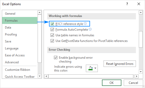
The below screenshot illustrates both the A1 and R1C1 reference styles:

To switch from the default A1 style to R1C1, click File > Options > Formulas, and then uncheck the R1C1 reference style box.
How to create a reference in Excel
To make a cell reference on the same sheet, this is what you need to do:
- Click the cell in which you want to enter the formula.
- Type the equal sign (=).
- Do one of the following:
- Type the reference directly in the cell or in the formula bar, or
- Click the cell you want to refer to.
- Type the rest of the formula and press the Enter key to complete it.
For example, to add up the values in cells A1 and A2, you type the equal sign, click A1, type the plus sign, click A2 and press Enter:

To create a range reference, select a range of cells on the worksheet.
For example, to add up the values in cells A1, A2 and A3, type the equal sign followed by the name of the SUM function and the opening parenthesis, select the cells from A1 through A3, type the closing parenthesis, and press Enter:

To refer to the whole row or entire column, click the row number or the column letter, respectively.
For instance, to add up all the cells in row 1, start typing the SUM function, and then click the header of the first row to include the row reference in your formula:

Tip. To get various information about a cell, use the CELL function.
How to change Excel cell reference in a formula
To change a cell address in an existing formula, carry out these steps:
- Click on the cell that contains the formula and press F2 to enter the Edit mode, or double-click the cell. This will highlight each cell/range referenced by the formula with a different color.
- To change a cell address, do any of the following:
- Select the reference in the formula and type a new one.
- Select the reference in the formula, and then select another cell or range on the sheet.

- To include more or fewer cells in a reference, drag the color-coded border of the cell or range.

- Press the Enter key.
How to cross reference in Excel
To refer to cells in another worksheet or a different Excel file, you must identify not only the target cell(s), but also the sheet and workbook where the cells are located. This can be done by using so-called external cell reference.
How to reference another sheet in Excel
To refer to a cell or a range of cells in another worksheet, type the name of the target worksheet followed by an exclamation point (!) before the cell or range address.
For example, here's how you can refer to cell A1 on Sheet2 in the same workbook:
=Sheet2!A1
If the name of the worksheet contains spaces or nonalphabetical characters, you must enclose the name within single quotation marks, e.g.:
='Target sheet'!A1
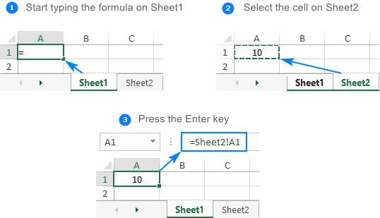
To prevent possible typos and mistakes, you can get Excel to create an external reference for you automatically. Here's how:
- Start typing a formula in a cell.
- Click the sheet tab you want to cross-reference and select the cell or range of cells.
- Finish typing your formula and press Enter.
For more information, please see How to reference cell in another worksheet in Excel.
How to reference another workbook in Excel
To refer to a cell or range of cells in a different Excel file, you need to include the workbook name in square brackets, followed by the sheet name, exclamation point, and the cell or a range address. For example:
=[Book1.xlsx]Sheet1!A1
If the file or sheet name contains non-alphabetical characters, be sure to enclose the path in single quotation marks, e.g.
='[Target file.xlsx]Sheet1'!A1
As with a reference to another sheet, you don't have to type the path manually. A faster way is to switch to the other workbook and select a cell or a range of cells there.
For the detailed guidance, please see How to reference cell in another workbook.
Relative, absolute and mixed cell references
There are three types of cell references in Excel: relative, absolute and mixed. When writing a formula for a single cell, you can go with any type. But if you intend to copy your formula to other cells, it is important that you use an appropriate address type because relative and absolute cell references behave differently when filled to other cells.
Relative cell reference in Excel
A relative reference is the one without the $ sign in the row and column coordinates, like A1 or A1:B10. By default, all cell addresses in Excel are relative.
When moved or copied across multiple cells, relative references change based on the relative position of rows and columns. So, if you want to repeat the same calculation across several columns or rows, you need to use relative cell references.
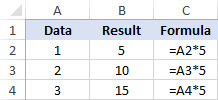
For example, to multiply numbers in column A by 5, you enter this formula in B2:
=A2*5
When copied from row 2 to row 3, the formula will change to:
=A3*5
For more information, please see Relative reference in Excel.
Absolute cell reference in Excel
An absolute reference is the one with the dollar sign ($) in the row or column coordinates, like $A$1 or $A$1:$B$10.
An absolute cell reference remains unchanged when filling other cells with the same formula. Absolute addresses are especially useful when you want to perform multiple calculations with a value in a specific cell or when you need to copy a formula to other cells without changing references.
For example, to multiply the numbers in column A by the number in B2, you input the following formula in row 2, and then copy the formula down the column by dragging the fill handle:
=A2*$B$2
The relative reference (A2) will change based on a relative position of a row where the formula is copied, while the absolute reference ($B$2) will always be locked on the same cell:

More details can be found in Absolute reference in Excel.
Mixed cell reference
A mixed reference contains one relative and one absolute coordinate, like $A1 or A$1.
There may be many situations when only one coordinate, column or row, should be fixed.
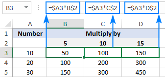
For example, to multiply a column of numbers (column A) by 3 different numbers (B2, C2 and D2), you put the following formula in B3, and then copy it down and to the right:
=$A3*B$2
In $A3, you lock the column coordinate because the formula should always multiply the original numbers in column A. The row coordinate is relative since it needs to change for other rows.
In B$2, you lock the row coordinate to tell Excel always to pick the multiplier in row 2. The column coordinate is relative because the multipliers are in 3 different columns and the formula should adjust accordingly.
As the result, all the calculations are performed with a single formula, which changes properly for each row and column where it is copied:
For real-life formula examples, please check out Mixed cell references in Excel.
How to switch between different reference types
To switch from a relative reference to absolute and vice versa, you can either type or delete the $ sign manually, or use the F4 shortcut:
- Double-click the cell that contains the formula.
- Select the reference you want to change.
- Press F4 to toggle between the four reference types.
Repeatedly hitting the F4 key switches the references in this order: A1 > $A$1 > A$1 > $A1.
Circular reference in Excel
In simple terms, a circular reference is the one that refers back to its own cell, directly or indirectly.
For example, if you put the below formula in cell A1, this would create a circular reference:
=A1+100
In most situations, circular references are a source of trouble and you should avoid using them whenever possible. In some rare case, however, they could be the only possible solution for a specific task.
The following tutorial explains how to find and remove circular references in Excel.
3D reference in Excel
3-D reference refers to the same cell or range of cells on multiple worksheets.
For example, to find an average of values in cells A1 to A10 in Sheet1, Sheet2 and Sheet3, you can use the AVERAGE function with a 3d reference:
=AVERAGE(Sheet1:Sheet3!A1:A3)
To make a formula with a 3d reference, here's what you need to do:
- Start typing a formula in a cell as usual, in this example we type =AVERAGE(
- Click the tab of the first sheet to be included in the 3d reference.
- Hold the Shift key and click the tab of the last sheet.
- Select the cell or range of cells to be calculated.
- Finish typing the formula and press the Enter key to complete it.
For more details, please see 3D reference in Excel.
Excel structured reference (table references)
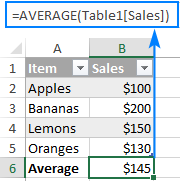
Structured reference is a special term for including table and column names in a formula instead of cells addresses. Such references can only be used for referring to cells in Excel tables.
For example, to find an average of numbers in the Sales column of Table1, you can use this formula:
=AVERAGE(Table1[Sales])
For more information, please see Structured refereces in Excel.
Excel names (named range)
An individual cell or a range of cells in Excel can also be defined by name. For this, you simply select a cell(s), type a name into the Name Box, and press the Enter key.
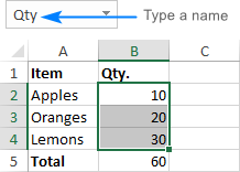
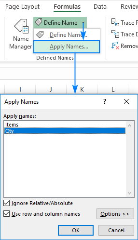
Upon creating new names, you may wish to replace the existing cell references in your formulas with the defined names. Here's how:
- Select the cells with the formulas in which you wish to change cell references to names.
To replace the references with defined names in all formulas on the active sheet, select any single blank cell.
- Go to the Formulas tab > Defined Names group, click the arrow next to Define Name, and then click Apply Names…
- In the Apply Names dialog box, select one or more names, and click OK.
As the result, the references in all or selected formulas will be updated to the corresponding names:
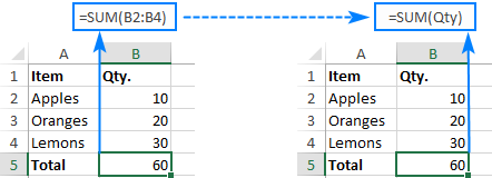
The detailed information on Excel names can be found in How to create and use a named range in Excel.
That's how you work with cell references in Excel. I thank you for reading and hope to see you on our blog next week!
 by
by
87 comments
Hi! This is a fantastically comprehensive guide, which makes me wonder if what I'm looking for is possible.
My work uses a spreadsheet for weekly planning, but some rules work across 2 weeks, eg 1 & 2, 3 & 4 (but never 2 & 3). This means that I have a setup for odd weeks and even weeks, but it's a nuisance to have to manually edit the cross-sheet formulae every time I create a new pair. Is there a way, for example, to reference "one sheet to the left"? So instead of an absolute sheet name in the reference, something like sheet(currentSheet.index-1)![Cell reference] ?
Thanks!
Hi! You can create a dynamic reference to a sheet using a value in a cell. This can be done using the INDIRECT function and these instructions: Creating an Excel dynamic reference to another sheet.
I am trying to create a set of calculations where multiple make reference to the cell above them. I trying to use OFFSET(INDIRECT(CELL("address")),-1,0)/RP[[#Totals],[Unit]] where RP is a named range and Unit is a column header. For some reason it only works once on a sheet. If I try to use it in a second cell it changes the the first to the out come of the second. Doing some error checking I found that when i enter a new =Cell("address"), no matter where it is in the sheet, all the previous incidences will always return the same value as the newest instance. Is there a way around this so that each =Cell("address") returns the correct value for that particular cell?
Hello Sam!
The CELL function always returns the address of the current cell, i.e., the last cell that was modified manually.
It always refers to the current cell, no matter how many times it is used on the sheet.
Read more: Excel CELL function with formula examples.
If you need to get address of different cells, use other functions like =ADDRESS(row, column) or =CELL("address", reference), where reference is a reference to a specific cell.
Unfortunately I can't offer you a solution as I don't really understand what you want to do. Explain it in more detail and I will try to help you.
Thank you for your formula
Hello,
I manually update the Income Statement each month by inputting figures to each account within each organizations by month. I need a formula that can update the new figures to the corresponding cells in the Income statement by organization, then month and finally to the respective account.
This formula ='[TB JULY GOV TEST COPY.xlsx]Table 1'!Q4 works to updates figures. However, the formula is not able to distinguish between organization, month, or account.
Roughly, this is what my Income Statement looks like:
Cell A1: Org. 1.01
Cell A2:A100: Account Numbers
Cell B1: Account description
Cells B2:N2: Jan – Dec
I can provide screenshot if necessary. Appreciate any insight you can provide. Thank you!
Hi! Your data is not very clear to me. I can guess that you can use the SUMIFS function and this guide to calculate the sum of the conditions: Excel SUMIFS and SUMIF with multiple criteria – formula examples.
Hi,
With vlookup formula, I could able to pull a value from another sheet.
Now I want to know from address/number of that cell from where the vlookup has brought the value.
Eg: In a table, there are values in 4 columns (column A, B, C & D) in sheet1.
In sheet2, I put a vlookup formula (with several conditions) in cell C2 with the reference of table in sheet1 and I got the answer as 500.
Now, I want to know the cell address of this 500 value which is in the table of sheet1.
In sheet1, in all the 4 columns the value lies in column D but I want to know the cell address of this 500.
Sorry for my english.
Thank you
Hi! If I understand your task correctly, try the following formula:
=CELL("address",INDIRECT("D"&ROW(D2)-1+MATCH(VLOOKUP(F1,A2:D20,4,FALSE),D2:D20,0)))
Read more: Excel CELL function with formula examples.
Sub Copy_Example()
Range("B1").Copy Destination:=Worksheets("Sheet1").Range("C1:C(G1)")
End Sub
I want to change the desired range every time based on the number inside the G1 cell? example G1=10 then c1:C10 OR G1=20 Then C1:C20 And ...
Your request goes beyond the advice we provide on this blog. If you have a specific question about a function or formula, I will try to answer it.
Good evening, this helped me incredibly!
I have a question still, it might be in here but I haven't been able to find it. The increasing a row each day from Pete Allen was close but not quite it. Apologies if I have skimmed over it and feel free to ask for more info if required.
I have a sheet where there are several individual cells that refers to a cell range which increases each day. Each is in their own respective column but not the same row.
As an example:
For the total of column A, yesterday's formula was =SUM(A82:A124), today it's =SUM(A82:A125) and tomorrow it'll be =SUM(A82:A126) and so on. There's at least a dozen other columns following the same format but the total of B is a few rows down so I cannot put absolute values for the top of the cell range, select the entire row and drag it down to copy and delete the former row.
Up until now I go through all the individual cells changing the last cell address of the cell ranges, the idea is to make them each refer to a single cell off the side so I only have to change the row number and they all change their formula's
Thank you for your time and thank you again in advance!
Hi! To avoid manually changing the formula when you add data, use a dynamic range as described in this guide: How to create and use dynamic named range in Excel.
You can also convert your data to an Excel table and refer to the columns of that table in the formula.
Hi I want to calculate value in first cell using formula with some reference cells and then keep answer, go to next cell use same formula with same reference cells but change data on reference cells without it affecting the first answer. please help
Hi! If two formulas refer to the same cells, both formulas will change. You can replace the first formula with its value using Paste Special.
hi uh i wanted to know how do i cell reference: All the cells of column A from row 2 to the end
Thanks
Hi! Type in cell = sign. Click the mouse to the first cell A2, and then press CTRL+SHIFT+DOWN ARROW to expand the selection to the last cell in the column. Press ENTER.
Thank
How can i reference a cell and return the specific character count of 789.
A1: 12/99/904
Ref: A1 and Return 904 Which would be characters 7 and 8 and 9.
I am only looking for specific characters of that code but they are specifically characters 789. The number will change.
Hi!
To extract a certain number of characters from text, use the MID function.
If I understand your task correctly, try the following formula:
=MID(A1,7,3)
Thank you very much this is exactly what i was lookin for. I am very appreciative. I have learned a new tool for my excel tool box.
I have a master workbook to track employee paid time off - one worksheet for each employee. Separately, each employee has a workbook with one worksheet for each year they have worked. I want the worksheet in the employees workbook to auto-update from the master workbook I update each pay period. How do I link those for a dynamic connection? This would be an exact copy of the sheet from the master workbook.
Hi!
The following tutorial should help: Excel reference to another sheet or workbook (external reference).
My Question:
Step 1: I want to get the cell address in another cell (eg: I got cell address as "C2" in "F2")
Step 2: I want to add some value to that cell address to create new cell address (eg: I want to add 4 to "C2" which is available in "F2" and new cell address "C6" to be placed in "G2")
Step 3: I want to get the value of the cell address which I made in another cell (eg: the value of "C6" to be placed in "H2")
Hi!
To get cell address in cell F2, use CELL function: =CELL("address",C2)
To create a dynamic link, use the INDIRECT function. =INDIRECT(F2)
To create a link to a cell that is four rows lower than the original cell, use the OFFSET function =OFFSET(INDIRECT(F2),4,0)
I hope I answered your question.
How can I find a value (CTRL+F) in second sheet, if the second sheet has referenced values from master sheet or workbook? How can I search for a specific value in displayed values of References?
I need to change the formula to reference cell below, please advise
=VLOOKUP((B3-DAY(B3)+1),'2468 - North Trust'!$A$15:$G$48,6,FALSE)
i am working to return a value from the a second sheet to a master sheet. The second sheet values changes every 10 rows as there is a calculation with the second sheet. I have used the cell reference but this becomes tedious when i have close to a 1000 records and manually changing each takes along a time. Is there a way to resolve this programmatically?
Master sheet Call A1 = Second sheet A1
Master sheet Call A2 = Second sheet A10
Master sheet Call A3 = Second sheet A20
Hi!
To create a dynamic cell reference, use the INDIRECT function.
=INDIRECT("Sheet2!A"&(ROW(A2)*10))
Thanks for your insightful guides!
i am making one dataset using excel: column A stores the (univoque) ID for each data, then links between data are expressed in term of this ID.
Assume the following:
Links are stored in column L (so L = A#, since ID's are in A)
Properties (say a,b,c for simplicity) are stored in column P (P = "a" or "b" or "c")
i would like to do something like this
if (property(link) == "a", "Prop_A",property(link) == "b", "Prop_B",property(link) == "c", "Prop_C")
so basically i would like to check the property of the structure LINKED to the original one, and then provide an attribute based on this to the original structure)
how can this be done?
i hope i was clear enough sorry but i'm hardly wrapping my head around this
Hi!
Your explanations are not very clear. I assume that you will find this article useful to find the data you need: Excel INDEX MATCH - formula examples
If this does not help, explain the problem in detail.
This was exactly it!
i was looking for IF (INDEX (MATCH (...));then,else)
thank you so much
Sir, Match function returns me a row number(for example 66), how to use this row number in another match function to refer B66. how can i call 66 in match(A2,B[66],0)
Hi!
To create a cell reference from a text string, use INDIRECT function.
I can't get the relative row reference to change across columns when I am using an IF statement. (it works outside of the IF statement)
For example:
=IF([Book1.xlsx]Sheet1!$A1="P","P","") when I copy ACROSS the columns, the row number doesn't change. It only changes if I copy DOWN the columns.
Is there something I can do instead of manually typing in all row number changes for each cell across the columns?
Hello!
The $ sign means that when you copy the formula, the column address will not change. For more information see this guide: Relative and absolute cell reference: why use $ in Excel formula.
Hi,
I am trying to cross reference two spread sheets so I can see a list of people that is not on one that is on the other. I am not sure how to go about this. What would my formula be?
Thank you!!
Hello!
To compare two columns in tables, you can use these formulas and guidelines.
To find unique values in two tables, use the special Compare Sheets tool. It is available as a part of our Ultimate Suite for Excel which contains over 60 new features and improvements.
Hey !
good afternoon.
I have such a problem
I have several google forms linked to Excel
I have a formula that has a total score across several forms. The main problem: when someone fills out these forms, my formula slides down 1 line. For example, if one person answered the form, his answer seems like inserted above, and the cell of the formula that was = B2 becomes C2. I've also tried writing a formula like = $B$2 - but it doesn't help me
Hello!
I recommend converting your data to an Excel table or using named ranges. In formulas, use references not to cells, but structured references in Excel table or to a named range.
Hello i have to increase cell reference by 200, so when you drag down a cell with a reference it will be increased by one (so A1--drag-> A2-->A3..) i have to increase 200( A1-->A201-->A401-->A601-...)
Sorry the bad english
Hello!
Use the ADDRESS function to create a cell reference. If the formula is written on row 1, then it looks like this:
=ADDRESS((1+(ROW()-1)*200),1)
I hope it’ll be helpful.
Very thanks
Hello I need to re-organie some boxes that have different vials. I need to put the coordantes of every cell so I know how it has been re arrange. Meaning that my cell A2(vial1) needs to go to B3(vial 1) with its coordanate and the text.
Is there any way to put a sub index with the coordante of every cell?
Thanks
Hi,
Can I combine two cells to reference a third cell.
for example - Cell A1 have a C in it cell A2 has a 2 in it.
Can I combine those two cells to produce an =C2 formula?
Hello!
Please check the formula below, it should work for you:
=INDIRECT(A1&A2)
Read more about the INDIRECT function in this article.
Hello,
Is there a way to use mixed cell references in excel when referring to another sheet?
For example:
I have a table I am filling in Sheet 2, I am using a formula that uses the reference 'Sheet1'!B13:B165.
When I go to flash fill the data in my table in Sheet 2, it changes to 'Sheet1'!B14:B166.
However, I need it to change just the columns it references in Sheet 1, not the rows.
I.E. I need to go from saying 'Sheet1'!B13:B165 in the 1st cell of the table to 'Sheet1'!C13:C165 in the 2nd cell in the table, then to 'Sheet1'!D13:D165 in the 3rd cell, etc.
Thus, is there a way to use a mixed cell reference when it's referring to cells in a different sheet?
Thank you!
Hello!
Here is the article that may be helpful to you: Excel mixed cell reference
It contains answers to your question.
Hi,
I have to add different cells of sheet 1 to sheet 2 like C1+C3+C5
For example:
Row A Row B Row C
Sl. No. Name pts
1 A 3
2 B 0
3 C 1
4 D 0
5 E 3
So next day when i filter the row c column with largest to smallest, the values should not change.
How to put the formula for this.
Hello!
I recommend replacing all formulas with values before sorting. Or make a copy of the table and sort it. Then your calculations will not change.
How do you pick a cell value that is the cross reference of a row and a column dependent on the text within the cell. For example if column A2 down had a list of names (i.e sally, harry, sue,tom etc) and row 1 had a list of fruit picked and the cells that align had the numbers of fruit picked against the name how do you select according to name and fruit? did that make sense?
Hello!
Please check out the following article on our blog, it’ll be sure to help you with your task: Vlookup based on row and column values.
You will be able to find the value at the intersection of the row and column.
the result of my funky formula being... =SHEET1!(B17)
I've got 778 work sheets, is there a way of getting the same cell of data from each work sheet in a list on a summary page without clicking through each work book.
For instance I want B17 on each work sheet in summary I want to columns headed Sheet and Product of B17 on each of the 778 sheets.
in Sheet 1 I want =B17
in Sheet 2 I want =B17
I've tried building formulas such as...
="="&"SHEET"&"CELLS WITH 1 to 778"&"!"&"B17"
Hello!
Please check out the following article on our blog, it’ll be sure to help you with your task: 3-D reference in Excel: reference the same cell or range in multiple worksheets.
I hope it’ll be helpful.
How do I write this formula in one sentence, "IF D4 is >=40 and F4 is >=40 and H4 is >=40 and J4 is >=40" so that, if the condition it true, the output will be "Pass" using IF(logic_test, [value_if_true] [value_if_false]) or any condition that will satisfy my request.
Thanks
=if(d4>=40,enter you want or if text use this "enter inside text ",if(f4>=40,enter you want or if text use this "enter inside text ",if(h4>=40,enter you want or if text use this "enter inside text ",if(j4>=40,enter you want or if text use this "enter inside text "))))
Hi, I'm not sure I know all the proper excel lingo, but here goes:
Can I convert a cell reference (only) within a formula to a value and keep the rest of the formula as is?
For example the value in A1 is 10, Column B formula is currently: +A1*2.9. I want to know if I can easily convert the formula in column B to: +10*2.9 - I need to keep the formula in column B, otherwise I would convert the formula to a value and be done with it! I have thousands of rows to convert and would rather not do it one by one. Thanks so much.
I want to reference another sheet (sheet 1) based on a number placed in a cell to represent the row on 'sheet 2 and call information based on the row given.
For example I place 11 in cell on sheet 2 then references various columns in that row.
11 must be constant for the row but the column data selected can change based on which column the required data is under.
Hello!
If I understand your task correctly, the following formula should work for you:
=INDIRECT(ADDRESS(Sheet2!$A$1,COLUMN(),2,1))
or
=INDIRECT("Sheet1!"&ADDRESS(Sheet2!$A$1,COLUMN(),2,1))
Cell Sheet2!$A$ contains 11.
Copy this formula to cells row by row.
I hope it’ll be helpful.
can u give me insights on these questions?
1. Why is it important to use cell reference or range of cells in creating a formula in text/sting functions?
2. Sate 2 common errors in inputting text function in Excel and their solution? give the error and present the solution step by step.
Thank you and hoping for a positive response:)
Hello!
You can learn more about references in this article: Relative and absolute cell reference: why use $ in Excel formula
Useful info here.
My problem is if Sheet1 has no value inputted in (ie) Cell A1 then the value in Sheet2 A1 is a 0. What do I use to make the formula in A1 of sheet2 a blank instead of a zero? My formula is ='Region'!A1
The entire 2nd sheet has references to the first sheet and they are working perfect except the blank value or no value on sheet1 is becoming zeros on sheet2.
So with columns A through BK and rows 1 through 110 I have an overload of zeros. Way too busy to focus on the numbers and words needed on the 9 tabs that reference sheet1 or tab1.
Any help is greatly appreciate.
Thank you
Hello!
I believe the following formula will help you solve your task:
=IF(A1<>"",A1,"")
Or use custom number format:
#,##0;-#,##0;
I hope this will help
I have a large sheet with at least 100 cell Names (that somehow got converted to A1 references). The method you show here is excellent but there doesn't seem to be a way of selecting ALL the names so they can replace ALL occurrences of their A1 references with their respective Names in the selected ramge.
hi, i got 1 master folder(A) contain 2 workbook(1 & 2).workbook 2,worksheet name 'sub' have link cell to workbook 1 worksheet name 'main'.the problem is when i copy this 2 workbook n paste it to new folder(sub 1 folder) the reference cell in workbook 2 stil refer to old reference location(master folder A).how can i make this copy workbook 1 & 2 follow new location (sub 1 folder) automatically after copy n paste?
Hello!
Excel does not automatically change links to external files. You need to keep track of this yourself.
Oh my! My original message was formatted so things made more since, but all the spaces were taken out and now it looks... confusing? I'll redo the part that is worst...
formula in A1 =(A107-A100)/A100
formula in A2 =(B107-B100)/B100
formula in A3 =(C107-C100)/C100 etc etc
Any way of having a variable in a cell reference? My setup is this... I have columns of numbers, 1 entry each day on each column, and display a 7-day average along the top row. But every day I have to change the formula for the 7-day avg of each column. Can I reference a cell location where I'd put the row# that changes from day to day?
Below, assume the last data entry is on line 107...
formula in A1 formula in A2 formula in A3
=(A107-A100)/A100 =(B107-B100)/B100 =(C107-C100)/C100 etc etc
The next day I have to change all the formulas, but only the row#'s change (incr by 1).
So, can the cell reference within the formula be written where the row# points to a cell location, which would contain the actual row# (107 & 100 in this case).
I tried many things, but they all result in error (assume reference cell is Z1 & Z2)...
=(A'Z1'-A'Z2')/A'Z2'
=(A(Z1)-A(Z2))/A(Z2)
=(A"Z1"-A"Z2")/A"Z2"
=(A[Z1]-A[Z2])/A[Z2] etc etc
I've run through all my guesses, and cannot find anything online addressing this. Maybe this can't be done, so I'll just have to add some more columns to my spreadsheet (already up to column DX, so this thing's unwieldy as it is :)
Thank you very much for taking the time to read this. If you somehow manage to understand what I'm asking, and have an answer, thank you even more!
Hello Pete!
You can use the INDIRECT function to specify the cell address. Your formula
=(A107-A100) / A100
can be written as
=(INDIRECT ("A" & D10) -INDIRECT ("A" & D11)) / INDIRECT ("A" & D11)
where cell D10 contains 107, cell D11 contains 100.
I hope this will help, otherwise please do not hesitate to contact me anytime.
Hi, I want to refer multiple cells in one cell how do I do it? Please reply
Hello!
For me to answer your question, please explain what references you’d like to make and for what purpose, what problem you want to solve? All types of cell references Excel allows to create are described in the above article. If you want to merge the content of several cells, please have a look at the other article on our blog:
https://www.ablebits.com/office-addins-blog/merge-combine-cells-excel/
I have 100 families with 1 to 7 family members and total nos. of families =100 and total members=450. I assigned sl.1 in C2 column for 1st family head(and no sl. number for other family members for the same family in C-column, so, C3&C4=blank if there are 3 family members). Again Sl.2 in C5 for 2nd family and so on. Now, in S-column I wrote ages of each members besides the name of respective members and in T-column, w.r.t. C2 row, I find 'height age' of each family by using formula T2=MAX(S2:S4)manually and T3,T4 kept blank as C3&C4 for 1st family. Here ranges of ages of different families will differ as per family size. Similarly, for 2nd family C5=2, T5=MAX(S5:S9)[C6 to C9 and T6 to T9 =remain blanks].I used following formula and drag-down it to avoid manual selection of each family group:"=IF(AND(C2>0,SUM(C2:C8)=C2),MAX(S2:S8),IF(AND(C2>0,SUM(C2:C7)=C2),MAX(S2:S7),IF(AND(C2>0,SUM(C2:C6)=C2),MAX(S2:S6),IF(AND(C2>0,SUM(C2:C5)=C2),MAX(S2:S5),IF(AND(C2>0,SUM(C2:C4)=C2),MAX(S2:S4),IF(AND(C2>0,SUM(C2:C3)=C2),MAX(S2:S3),IF(AND(C2>0,C3>0),MAX(S2:S2),"")))))))". I think there is more appropriate formula.Please help me out.
Hello Biswajit!
I'm sorry, it is not very clear what result you want to get. Could you please describe your task in more detail and send us a small sample workbook with the source data and expected result to support@ablebits.com? Please shorten your tables to 10-20 rows/columns and include the link to your blog comment.
We'll look into your task and try to help.
Hello! Very useful information, I just cannot figure out how to "update this cell to read Support to make it consistent with the other tables" does anyone have any idea what that means? it says it with a red arrow on the top right corner of the specific cell. I'd appreciate some help!
Hey I have a problem. In cell D4 I put a value "50"and D4 is formatted as "Percentage" so it's showing as "50%". Now in another cell(B4) I want D4 as reference, so I combine text and cell reference as "="Less: Depreciation @"&D4"(first double quote not in formula) and it giving the result in B4 is "Less: Depreciation @0.5" but I want it should be "Less: Depreciation @50%" and also D4 should be "50%". Any suggestion would be very appreciated. Thanks in advance.
I have 3 sheets.
In sheet 1 column A may hold a value, it can be empty too.
In sheet 2 column A references column A of sheet 1. If column A in sheet 1 is empty, column A in sheet 2 will show no value, it will however contain the reference. So technically it is not empty, functionally it is empty.
In sheet 3 I want to test if column A of sheet 2 is empty.
What formula could I use best?
For my bookkeeping I count the expensives in a worksheet "wk 1", "wk 2", "wk 3", "wk 4" & "wk 5A" as an example for January. Week 5A is not a full week and in February I begin with "wk 5B". After week 5A I make a summary "JAN" of all the week totals and monthly fixed amounts like subscription fees, cable TV, internet, etc.
The week totals are always at cell E12. To get that value I have a cell with ='wk 1'!$E$12 and it works, but I want to make it easier for my wife, so she can copy the sheets at to end tab herself. Hence I have a column with "wk 1" to "wk 5A" (cells A4 to A8) she has to fill in, but I can't get the formula using these values to work for cells B4 to B8. I need for cell B4 something like ="'"&A4&"'!"$E$12 but it doesn't work.
I have solved the problem after more digging. The INDIRECT formula wasn't working properly as it didn't accept the E12 cell reference. With aid of ADDRESS (row 12, column 5) it worked. So, the formulas for B4 to B8 are:
=INDIRECT(ADDRESS(12,5,1,1,A4))
=INDIRECT(ADDRESS(12,5,1,1,A5))
etc.
Thank you,
I have a question I will ask it as an example:
I have two columns A and B (as if I want to plot them in a graph). I want to extract the maximum value of the column A so I used the formula =MAX(A1:A5000) {for example}. Now I want to extract the respective value in column B and I do not know how. For example if the maximum value is located in A2000 I want in another cell to have the value of B2000.
Thank you in advance
you should use a search formula for this. such as:
=search(C1;A:A;B:B)
Being C1=MAX(A1:A5000)
or
=Vlookup(C1;A1:B5000;2)
Hi Svetlana,
Can we use Cell name in formula instead of reference, like I have a cell name "Exchange_rate" and I want to link another cell with this one and in formula bar showing name "Exchange_rate" instead of Cell reference like A1 etc.
You can put the cell name into the Names box. In the above example a cell range was used QTY and later a formula =SUM(QTY)
Thank you!
A little question: (...For example, the range A1:C2 includes 9 cells from A1 through C2...). Nine cells or six?
Hi Vladimir,
Surely, 6 cells. Thank you, fixed :)
thanks a lot , I learn vary important information from this web. It helped me in my work.
Good