The tutorial provides a list of Excel basic formulas and functions with examples and links to related in-depth tutorials.
Being primarily designed as a spreadsheet program, Microsoft Excel is extremely powerful and versatile when it comes to calculating numbers or solving math and engineering problems. It enables you to total or average a column of numbers in the blink of an eye. Apart from that, you can compute a compound interest and weighted average, get the optimal budget for your advertising campaign, minimize the shipment costs or make the optimal work schedule for your employees. All this is done by entering formulas in cells.
This tutorial aims to teach you the essentials of Excel functions and show how to use basic formulas in Excel.
The basics of Excel formulas
Before providing the basic Excel formulas list, let's define the key terms just to make sure we are on the same page. So, what do we call an Excel formula and Excel function?
- Formula is an expression that calculates values in a cell or in a range of cells.
For example,
=A2+A2+A3+A4is a formula that adds up the values in cells A2 through A4. - Function is a predefined formula already available in Excel. Functions perform specific calculations in a particular order based on the specified values, called arguments, or parameters.
For example, instead of specifying each value to be summed like in the above formula, you can use the SUM function to add up a range of cells: =SUM(A2:A4)
You can find all available Excel functions in the Function Library on the Formulas tab:

There exist 400+ functions in Excel, and the number is growing by version to version. Of course, it's next to impossible to memorize all of them, and you actually don't need to. The Function Wizard will help you find the function best suited for a particular task, while the Excel Formula Intellisense will prompt the function's syntax and arguments as soon as you type the function's name preceded by an equal sign in a cell:
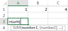
Clicking the function's name will turn it into a blue hyperlink, which will open the Help topic for that function.
Tip. You don't necessarily have to type a function name in all caps, Microsoft Excel will automatically capitalize it once you finish typing the formula and press the Enter key to complete it.
10 Excel basic functions you should definitely know
What follows below is a list of 10 simple yet really helpful functions that are a necessary skill for everyone who wishes to turn from an Excel novice to an Excel professional.
SUM
The first Excel function you should be familiar with is the one that performs the basic arithmetic operation of addition:
In the syntax of all Excel functions, an argument enclosed in [square brackets] is optional, other arguments are required. Meaning, your Sum formula should include at least 1 number, reference to a cell or a range of cells. For example:
=SUM(B2:B6) - adds up values in cells B2 through B6.
=SUM(B2, B6) - adds up values in cells B2 and B6.
If necessary, you can perform other calculations within a single formula, for example, add up values in cells B2 through B6, and then divide the sum by 5:
=SUM(B2:B6)/5
To sum with conditions, use the SUMIF function: in the 1st argument, you enter the range of cells to be tested against the criteria (A2:A6), in the 2nd argument - the criteria itself (D2), and in the last argument - the cells to sum (B2:B6):
=SUMIF(A2:A6, D2, B2:B6)
In your Excel worksheets, the formulas may look something similar to this:

Tip. The fastest way to sum a column or row of numbers is to select a cell next to the numbers you want to sum (the cell immediately below the last value in the column or to the right of the last number in the row), and click the AutoSum button on the Home tab, in the Formats group. Excel will insert a SUM formula for you automatically.
Useful resources:
AVERAGE
The Excel AVERAGE function does exactly what its name suggests, i.e. finds an average, or arithmetic mean, of numbers. Its syntax is similar to SUM's:
Having a closer look at the formula from the previous section (=SUM(B2:B6)/5), what does it actually do? Sums values in cells B2 through B6, and then divides the result by 5. And what do you call adding up a group of numbers and then dividing the sum by the count of those numbers? Yep, an average!
The Excel AVERAGE function performs these calculations behind the scenes. So, instead of dividing sum by count, you can simply put this formula in a cell:
=AVERAGE(B2:B6)
To average cells based on condition, use the following AVERAGEIF formula, where A2:A6 is the criteria range, D3 is he criteria, and B2:B6 are the cells to average:
=AVERAGEIF(A2:A6, D3, B2:B6)

Useful resources:
MAX & MIN
The MAX and MIN formulas in Excel get the largest and smallest value in a set of numbers, respectively. For our sample data set, the formulas will be as simple as:
=MAX(B2:B6)
=MIN(B2:B6)

Useful resources:
COUNT & COUNTA
If you are curious to know how many cells in a given range contain numeric values (numbers or dates), don't waste your time counting them by hand. The Excel COUNT function will bring you the count in a heartbeat:
While the COUNT function deals only with those cells that contain numbers, the COUNTA function counts all cells that are not blank, whether they contain numbers, dates, times, text, logical values of TRUE and FALSE, errors or empty text strings (""):
For example, to find out how many cells in column B contain numbers, use this formula:
=COUNT(B:B)
To count all non-empty cells in column B, go with this one:
=COUNTA(B:B)
In both formulas, you use the so-called "whole column reference" (B:B) that refers to all the cells within column B.
The following screenshot shows the difference: while COUNT processes only numbers, COUNTA outputs the total number of non-blank cells in column B, including the the text value in the column header.

Useful resources:
IF
Judging by the number of IF-related comments on our blog, it's the most popular function in Excel. In simple terms, you use an IF formula to ask Excel to test a certain condition and return one value or perform one calculation if the condition is met, and another value or calculation if the condition is not met:
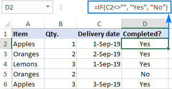
For example, the following IF statement checks if the order is completed (i.e. there is a value in column C) or not. To test if a cell is not blank, you use the "not equal to" operator ( <>) in combination with an empty string (""). As the result, if cell C2 is not empty, the formula returns "Yes", otherwise "No":
=IF(C2<>"", "Yes", "No")
Useful resources:
TRIM
If your obviously correct Excel formulas return just a bunch of errors, one of the first things to check is extra spaces in the referenced cells (You may be surprised to know how many leading, trailing and in-between spaces lurk unnoticed in your sheets just until something goes wrong!).
There are several ways to remove unwanted spaces in Excel, with the TRIM function being the easiest one:
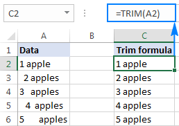
For example, to trim extra spaces in column A, enter the following formula in cell A1, and then copy it down the column:
=TRIM(A1)
It will eliminate all extra spaces in cells but a single space character between words:
Useful resources:
LEN
Whenever you want to know the number of characters in a certain cell, LEN is the function to use:
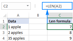
Wish to find out how many characters are in cell A2? Just type the below formula into another cell:
=LEN(A2)
Please keep in mind that the Excel LEN function counts absolutely all characters including spaces:
Want to get the total count of characters in a range or cells or count only specific characters? Please check out the following resources.
Useful resources:
AND & OR
These are the two most popular logical functions to check multiple criteria. The difference is how they do this:
- AND returns TRUE if all conditions are met, FALSE otherwise.
- OR returns TRUE if any condition is met, FALSE otherwise.
While rarely used on their own, these functions come in very handy as part of bigger formulas.
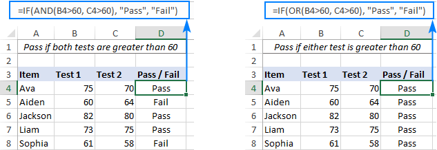
For example, to check the test results in columns B and C and return "Pass" if both are greater than 60, "Fail" otherwise, use the following IF formula with an embedded AND statement:
=IF(AND(B2>60, B2>60), "Pass", "Fail")
If it's sufficient to have just one test score greater than 60 (either test 1 or test 2), embed the OR statement:
=IF(OR(B2>60, B2>60), "Pass", "Fail")
Useful resources:
CONCATENATE
In case you want to take values from two or more cells and combine them into one cell, use the concatenate operator (&) or the CONCATENATE function:
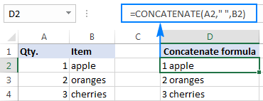
For example, to combine the values from cells A2 and B2, just enter the following formula in a different cell:
=CONCATENATE(A2, B2)
To separate the combined values with a space, type the space character (" ") in the arguments list:
=CONCATENATE(A2, " ", B2)
Useful resources:
TODAY & NOW
To see the current date and time whenever you open your worksheet without having to manually update it on a daily basis, use either:
=TODAY() to insert the today's date in a cell.
=NOW() to insert the current date and time in a cell.
The beauty of these functions is that they don't require any arguments at all, you type the formulas exactly as written above.

Useful resources:
Best practices for writing Excel formulas
Now that you are familiar with the basic Excel formulas, these tips will give you some guidance on how to use them most effectively and avoid common formula errors.
Do not enclose numbers in double quotes
Any text included in your Excel formulas should be enclosed in "quotation marks". However, you should never do that to numbers, unless you want Excel to treat them as text values.
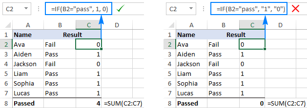
For example, to check the value in cell B2 and return 1 for "Passed", 0 otherwise, you put the following formula, say, in C2:
=IF(B2="pass", 1, 0)
Copy the formula down to other cells and you will have a column of 1's and 0's that can be calculated without a hitch.
Now, see what happens if you double quote the numbers:
=IF(B2="pass", "1", "0")
At first sight, the output is normal - the same column of 1's and 0's. Upon a closer look, however, you will notice that the resulting values are left-aligned in cells by default, meaning those are numeric strings, not numbers! If later on someone will try to calculate those 1's and 0's, they might end up pulling their hair out trying to figure out why a 100% correct Sum or Count formula returns nothing but zero.
Don't format numbers in Excel formulas
Please remember this simple rule: numbers supplied to your Excel formulas should be entered without any formatting like decimal separator or dollar sign. In North America and some other countries, comma is the default argument separator, and the dollar sign ($) is used to make absolute cell references. Using those characters in numbers may just drive your Excel crazy :) So, instead of typing $2,000, simply type 2000, and then format the output value to your liking by setting up a custom Excel number format.
Match all opening and closing parentheses
When crating a complex Excel formula with one or more nested functions, you will have to use more than one set of parentheses to define the order of calculations. In such formulas, be sure to pair the parentheses properly so that there is a closing parenthesis for every opening parenthesis. To make the job easier for you, Excel shades parenthesis pairs in different colors when you enter or edit a formula.
Copy the same formula to other cells instead of re-typing it
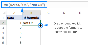
Once you have typed a formula into a cell, there is no need to re-type it over and over again. Simply copy the formula to adjacent cells by dragging the fill handle (a small square at the lower right-hand corner of the cell). To copy the formula to the whole column, position the mouse pointer to the fill handle and double-click the plus sign.
Note. After copying the formula, make sure that all cell references are correct. Cell references may change depending on whether they are absolute (do not change) or relative (change).
For the detailed step-by-step instructions, please see How to copy formulas in Excel.
How to delete formula, but keep calculated value
When you remove a formula by pressing the Delete key, a calculated value is also deleted. However, you can delete only the formula and keep the resulting value in the cell. Here's how:
- Select all cells with your formulas.
- Press Ctrl + C to copy the selected cells.
- Right-click the selection, and then click Paste Values > Values to paste the calculated values back to the selected cells. Or, press the Paste Special shortcut: Shift+F10 and then V.
For the detailed steps with screenshots, please see How to replace formulas with their values in Excel.
Make sure Calculation Options are set to Automatic
If all of a sudden your Excel formulas have stopped recalculating automatically, most likely the Calculation Options somehow switched to Manual. To fix this, go to the Formulas tab > Calculation group, click the Calculation Options button, and select Automatic.
If this does not help, check out these troubleshooting steps: Excel formulas not working: fixes & solutions.
This is how you make and manage basic formulas in Excel. I how you will find this information helpful. Anyway, I thank you for reading and hope to see you on our blog next week.
 by
by
410 comments
Really helpful information.
Thank you, the explanation is easy to understand.
Hello Please provide me PDF File Excel Formula Basic to all excel formula
Really helpful information
I want Vlookup formula please send
I recommend reading this guide: Excel VLOOKUP function tutorial with formula examples
Nice
please help me
5000 to 10000 equal to1 point
10001 to 20000 equal to 2 point
equation please
Hi!
I recommend reading this guide: Nested IF in Excel – formula with multiple conditions. It covers your case completely.
Hi,
I have Three figures Cell A1-Cell A2 result in cell A3. What I'm trying to do is , if the resulting figure in Cell A3 is positive then it should be displayed in Cell A4, if it's a negative number it should be in A5?
Any help would be most appreciated!
Thank You.
Brian.
Hi!
You can find the answer to your question in this article: IF formula for numbers.
it's good than other websites
=((D9/J9))^(1/IF(AND(H9<G9;B9<A9));MIN(I9;C9);5,284))
what are 5 and 284
can anyone explain this formula?
Hi there, I have an excel sheet in which there are 95 records that is rows. and six columns. In the first row, first column is for the name of the student and the rest 5 columns contain five subject name.
Rest 94 rows contains the name and the marks of the student corresponding to the subject.
I want to give different names to these 94 rows. And the condition is that the name of the row should be the name of the student.
Could you please tell me the solution.
Hello!
If I understand your task correctly, here is the article that may be helpful to you: Excel named range - how to define and use names in Excel.
I hope my advice will help you solve your task.
Thank you! I got the solution.
Hi there, I have a sheet of 5th standard final report card. In which I have 60 student and 6 subject. I have the marks of all the students of all the subjects . I want to know the highest marks of a particular student just by entering the name of student. And the subject in which the student got the highest marks and the marks (highest) should be shown. Could you please tell me the formula for this query.
Thank you in advance.
Hello!
If the student's name is written in cell K1, then you can get his maximum mark and subject using the following formulas:
=MAX(FILTER(B2:G10,A2:A10=K1))
=INDIRECT(ADDRESS(1,MATCH(MAX(FILTER(B2:G10,A2:A10=K1)), FILTER(B2:G10,A2:A10=K1),0)+1))
You can learn more about FILTER function in Excel in this article on our blog.
Thank you!
There are 7 columns.
1Adm No
2 Name
3 Fee structure
4 Received Fee
5 Pending Fee
6 Paper Money
7 Admission Fee
I want to seperate those students whose fee is pending. Adm No ,Students Name and pending fee these three columns i want to automatically move another sheet .
Which formula wil be apply .
Hello!
To conditionally retrieve data, you can use the FILTER function.
=FILTER(A1:E100,E1:E100 > 0)
Or you can copy the data to another sheet and use the Excel Filter tool.
I hope it’ll be helpful. If something is still unclear, please feel free to ask.
How to write this in excel
Price divide by 1.16 minus 40%
Hi!
Here is the article that may be helpful to you: How to calculate percentage in Excel.
i had came across a spreadsheet were it has a table with titles that doesn't change when you flip a page, typing a specific year to a assign field that it is already navigated by the developer of the template..... i am working on a spreadsheet recording salary for a corporation, and i was wondering if only you can help me create a task to a cell that only act like flipping pages within the same worksheet were default information remain along while the information reflect the change when data are enter and falls in specific time range that is assign to each page.
This template I'm referring to is something to do with a Budget vs Actual template.
Hi!
I can help you write the formula if you describe the problem more accurately and concisely.
I want set a maximum number like 3, where any value which greater than 3 it become into 3. Is it possible ?
Hello!
If I understood the problem correctly, you can use the IF function.
IF(A1>3,3,A1)
How I can with the same cell to for varying cell. I need the syntax. Example: I3*C17+I4*D17+I5*E17+I6*F17+I7*G17+I8*H17 the I3, I4 .... I8 I don't want to vary when their multiplier varies from cell to cell.
Regards,
Hello!
If I understand your task correctly, the following formula should work for you:
=SUMPRODUCT(I3:I7,TRANSPOSE(C17:G17))
=IF(MONTH(DATE((RIGHT(A1,4))+1,2,29))=2,DATE((RIGHT(A1,4))+8,1,1)+((MID(A1,4,2))*30-120+(LEFT(A1,2))-22),DATE((RIGHT(A1,4))+8,1,1)+((MID(A1,4,2))*30-120+(LEFT(A1,2))-23))
what wrong with this formula? I can not fix the error.
Hello!
Write an example of the source data and the result you want to get.
What is the formula to always add the same cell as you draw down a column? eg. Wish to add the value in A1 after the cell has calculated a formula and be able to see the difference down the list if I change the single value in A1
Example:
Cell A3=A2+A1
Cell A4=A3+A1
Cell A5=A4+A1.......down to cell A700
Hello!
If I understand your task correctly, the following formula should work for you:
=A2+$A$1
Please check out this article to learn how to use $ in Excel formula
Thankyou, this is exactly what I asked for. 10/10
I have two spread sheet one of i yellow collar highlighted one of my active partner name and business registration number , other spread. sheet desperately are include all businesses name , now i want second spread sheet category a active and inactive , how i can get first spread sheet detail collared name as machine in to second sheet
Hello!
Using the Select by color utility, you can select all the cells highlighted with a certain color and then copy them to another sheet. It is available as a part of our Ultimate Suite for Excel that you can install in a trial mode and check how it works for free: https://www.ablebits.com/files/get.php?addin=xl-suite&f=free-trial
If this is not what you wanted, please describe the problem in more detail.
how to adjustment of per rate formula in excel
Hello!
Here is the article that may be helpful to you: Excel RATE function, formula examples to calculate interest rate
I hope it’ll be helpful.
I want to show grace marks obtained by a student in the marksheet along with the grace marks symbol. Ex. 30+3
33+
Great site. Cheers for posting.
HELLO,
wanted help in how u gonna write a formula for summing the total of mark up to 100 buh prompting the user on a total score greater than 100 and less than zero
i have a problem, when i want to write a formula to add marks to the average scored of student who scored 44 (included) and 50 ( excluded) to get new average
Hello!
I’m sorry but your task is not entirely clear to me.
Please describe your problem in more detail. Include an example of the source data and the result you want to get. It’ll help me understand your request better and find a solution for you
how to count name from different sheet in excel
Hello!
Please have a look at this article — Excel reference to another sheet or workbook (external reference)
I hope this will help
WHAT IS THE CORRECT EXCEL FORMULA FOR CELL M16…M27 TO CALCULATE THE NET DISCOUNT
Hi,
Please describe your problem in more detail. It’ll help me understand it better and find a solution for you.
I didn't like these examples
Hi,
Have you tried the ways described in this blog post? If they don’t work for you, then please describe your task in detail, I’ll try to suggest a solution.
I want to know 475 formulas of excel
But its help me a lot thank you for it
Thanks for sending? from ??
It really helps me to do my IT practicle file
Hi,
I am not sure I fully understand what you mean.
Could you please describe it in more detail? What result do you want to get?
Noice and nice
Hi
I m using excell in office but i want to save formula for name displaying system. For eg (By typing its pan number it should display its name saved in excell in next column) please help me
Thank You
MF:( i don't know how to use excel:((((((((((
200 100 = 100
300 400 = -100 300-400=0 Passible
400 300 = 100
500 600 = -100
Hello!
Sorry, I do not fully understand the task. Could you please describe it in more detail? What result do you want to get? Thank you!
I'm looking for a formula to calculate National Insurance payments please-
Under £183 = 0%
£183.01- £962 = 12%
£962.01+ = 2%
Im thinking SUMPRODUCT but getting lost, Thank you
Hello!
For me to be able to help you better, please describe your task in more detail. I cannot know how these payments are made. Please specify what you were trying to find, what formula you used and what problem or error occurred. Give an example of the source data and the expected result.
It’ll help me understand it better and find a solution for you.
300-500=0
Good day.
I have a spread sheet of 300+ line. I want to add a formula what hides values what is the same amount, but opposite (positive and negetive).
A1 -35,00
B1 -34,80
C1 -33,26
D1 -15,00
E1 32,12
F1 33,26
G1 34,80
Example:
A1 - Stay
(B1,G1) Hide
(C1,F1) Hide
D1 - Stay
E1 - Stay
Thank you
Hello!
You haven't specified exactly how you want to hide the values. However, you can use conditional formatting in your table.
Use condition formula
=SUM(--(1:1=-A1))=1
For this condition, you can set the font color to white in the cell.
How can I get only numerical numbers from text.
Examples:-
Hi please check 54618464
51856792 requirements cleared
Please check 3192675 and confirm
Hello!
Please read my answer to this comment.
Hi,Kindly guide me
In column K check condition 1,2,3,4 then get value from column H and sum value below another table according to 1,2,3,4
Hello!
I’m sorry but your task is not entirely clear to me. For me to be able to help you better, please describe your task in more detail. Please specify what you were trying to find, what formula you used and what problem or error occurred. Give an example of the source data and the expected result.
It’ll help me understand it better and find a solution for you.
GOOD DAY
COULD SOMEONE PLEASE ASSIST ME.
i AM TRYING TO WORK OUT A FORMULA PLEASE SEE BELOW.
PART DESCRIPTION PART NUMBER QTY UNIT PRICE DISCOUNT SUB TOTAL
BULB 2 R50 15% R85
SO HOW DO i WORK OUT THE FORMULA TO SAY R50 X 2 -15% WILL = R85.
I have one Excel marklist that displays marks out of 100 in all subjects(10 subjects). I want to reduce all marks in the marklist to half.how can i do that for entire marklist.pls reply urgent
Hi
I new to Excel and being a complete Brain Dead moment i am trying to do a balance sheet,and I just cant seem to get old ballance showing new ballance value. It's a simple spreadsheet where:
I have 3 columns.
B2 is current balance £100
C2 is Payment £30
D2 is Balance £70
BUT I then want B2 to show new ballance D2.
Ie: B2 is Owing £100 C2 is I pay £30. D2 NEW BALANCE of £70. Then B2 shows new ballance of D2 £70.
Hope this helps and thank you
Pete
lots of time taken while reading ,but it's more useful when work in excel with your tips to reduce working time ...thanks for sharing the valuble one..
"Your students have completed their oral and written exams and you need to get their grade. If they received greater than or equal to 85 in both parts they will get a grade of A otherwise the grade is a Pass.
Create the formula you would enter."
Can you help me create this formula?
Thank you for your help.
Hello!
I’m sorry but your task is not entirely clear to me.
Please describe your problem in more detail. Include an example of the source data and the result you want to get. It’ll help me understand your request better and find a solution for you. Thank you.
=+Sheet1!D7 what does it mean
I'm trying to error proof an excel sheet. I need for the input be between 113.5 to 116.5. if it falls in-between that range then it's ok, if not then it highlights that cell in red.
Hello Averon!
You need to use conditional formatting. I recommend studying this article on conditional formatting on our blog.
hello Please provide me PDF File Excel Formula Basic to all excel formula
If there are number of releatative items in column. Ex.
A 1
B 3
A 5
C 1
D 3
B 2
I want to make column of from above data like
A
B
C
D
What does the at (@) symbol do in a formula?
Hi Larry,
The @ symbol is used in structured references (table references) to refer to cells in the same row where the formula is. Typically, the @ character is followed by the column name.
For example, the following formula adds up numbers in the "South" and "West" columns of the current row in the table named "Regions":
=SUM(Regions[@South], Regions[@West])
For more information, please see How to use structured references in Excel tables.
I love that, they are all interested.