Want to know how many characters there are in a certain cell? This tutorial will help you choose an Excel formula for character count best suited for your particular case.
Initially, Excel was designed to work with numbers. Fortunately, the developers of this helpful application didn't forget about text. Below, you'll find a number of formulas for counting characters in Excel. Just look through the examples and see which one best suits your needs.
Here are the cases we are going to cover:
Excel formula to count the number of characters in a cell
First things first, let's solve the most common case. To find how many characters there are in an Excel cell, the formula is as simple as:
For example, to count characters in each cell of column A beginning in A3, this is what you need to do:
- Enter the below formula in any empty cell in row 3:
=LEN(A3) - Double-click the fill handle to get the formula copied across the whole column.
Done!
Feel free to use this formula each time you need to count the number of characters in a string.
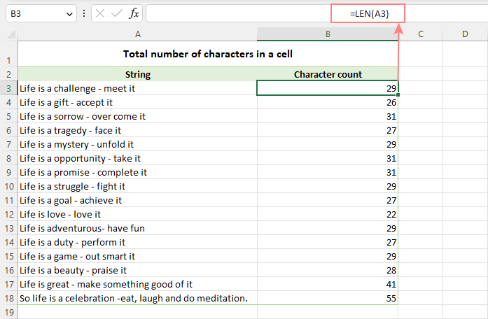
Note. Please pay attention that the Excel LEN function counts absolutely all characters in a cell, including letters, numbers, punctuation marks, special symbols, and all spaces (leading, trailing and spaces between words).
Count characters in a range of cells
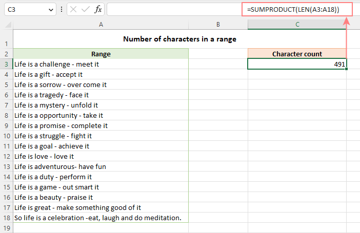
To get the total of characters in an Excel range, you can use the LEN function together with SUMPRODUCT:
And your real-life formula may look similar to this:
=SUMPRODUCT(LEN(A3:A18))
Another way to count all characters in a range is using LEN in combination with the SUM function:
=SUM(LEN(A3:A18))
Unlike SUMPRODUCT, the SUM function does not process arrays by default, so you need to press Ctrl + Shift + Enter to turn it into an array formula in Excel 2019 and earlier. In Excel 365 and 2021, it works as a regular formula due to inbuilt support for dynamic arrays.
How this formula works:
The logic is very simple. The LEN function calculates the string length for each individual cell in the specified range and returns an array of numbers. And then, SUMPRODUCT or SUM adds up those numbers and returns the total character count.
How to count specific characters in a cell
To find out how many times a given character appears in a cell, the generic formula is:
Suppose you maintain a database of items where each item type has its own unique identifier. And each cell contains several items separated by comma, space, or any other delimiter. The task is to get the number of occurrences of a certain unique identifier in each cell.
Assuming the list of items is in column A beginning in A3, and the target character is in column B in the same row, the formula is as follows:
=LEN(A3) - LEN(SUBSTITUTE(A3, B3, ""))
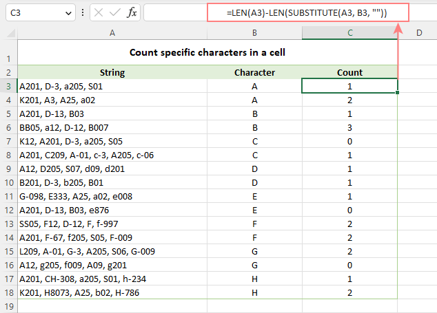
Note. Excel's SUBSTITUTE is a case-sensitive function, and therefore the above formula treats uppercase and lowercase letters as different characters. For example, cell A4 in the screenshot above contains one occurrence of "a" and two occurrences of "A". The formula counted only the uppercase "A" and returned 2 as the result.
How this formula works:
To understand the formula's logic, let's break it down into smaller parts:
- First, you find the total string length in cell A3 with:
LEN(A3) - Then, you remove all occurrences of the letter "A" in A3 by replacing it with an empty string:
SUBSTITUTE(A3, "A", "") - The next step is to find the string length without the letter "A":
LEN(SUBSTITUTE(A3, "A", "")) - Finally, you subtract the length of the string without "A" from the total length string:
LEN(A3) - LEN(SUBSTITUTE(A3, B3, ""))
As the result, you get the count of "removed" characters, which is the number of occurrences of that particular character in the cell.
Case-insensitive formula to count letters in Excel cell
When counting letters in Excel cells, you may sometimes need a formula that ignores the letter case. To make such a formula, use the UPPER function inside SUBSTITUTE to convert a given letter to uppercase before running the substitution.
For example, to count both "A" and "a" in cell A3, use this formula:
=LEN(A3) - LEN(SUBSTITUTE(UPPER(A3), "A", ""))
The LOWER function will also do:
=LEN(A3) - LEN(SUBSTITUTE(LOWER(A3), "a", ""))
A slightly more complex way is using nested SUBSTITUTE functions:
=LEN(A3) - LEN(SUBSTITUTE(SUBSTITUTE (A3, "A", ""), "a", "")
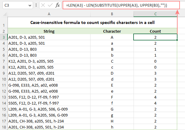
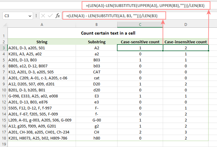
In our data set, the letters to be counted are input in column B, so we convert both the source cell and the cell containing the character to uppercase:
=LEN(A3) - LEN(SUBSTITUTE(UPPER(A3), UPPER(B3),""))
And this works beautifully irrespective of the target letter's case:
How to count certain text/substring in a cell
If you want to know how many times a certain combination of characters appears in a given cell (e.g. "C2" or "C-2" or "cat"), then divide the characters count by the length of the substring.
Case-sensitive formula:
=(LEN(A3) - LEN(SUBSTITUTE(A3, B3, ""))) / LEN(B3)
Case-insensitive formula:
=(LEN(A3)-LEN(SUBSTITUTE(UPPER(A3), UPPER(B3),""))) / LEN(B3)
Where A3 is the original text string and B3 is the substring to count.
For the detailed explanation of the formula, please see How to count specific text / words in a cell.
How to count specific characters in a range
Knowing a formula for counting certain characters in a single cell, it's quite easy to modify it a little further to count the number of occurrences of a given character in several cells. For this, just place the LEN formula inside the SUMPRODUCT function that can handle arrays:
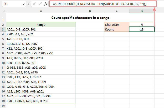
For example, to get to know how many times the character in D2 occurs in the range A3:A18, the formula is:
=SUMPRODUCT(LEN(A3:A18) - LEN(SUBSTITUTE(A3:A18, D2, "")))
Instead of SUMPRODUCT, you can also use SUM:
=SUM(LEN(A3:A18) - LEN(SUBSTITUTE(A3:A18, D2, "")))
But this formula requires pressing Ctrl + Shift + Enter because, in all versions other than Excel 365 and 2021, SUM can handle arrays only in an array formula.
How this formula works:
The SUBSTITUTE function replaces all occurrences of a given character ("A" in this example) with an empty string ("").
The text string returned by SUBSTITUTE is served to the LEN function so it calculates the string length without A's.
The string length without A's is subtracted from the total length of the original string. The result is an array of character counts per cell.
Finally, SUMPRODUCT sums the numbers in the array and returns the total character count in the range.
Case-insensitive formula to count letters in a range
To create a case-insensitive formula for counting specific characters in a range, follow the same approaches that we used for counting certain letters in a cell regardless of the text case.
Use the UPPER function and supply an uppercase letter:
=SUMPRODUCT(LEN(A3:A18) - LEN(SUBSTITUTE(UPPER(A3:A18), "A", "")))
Use the LOWER function and supply a lowercase letter:
=SUMPRODUCT(LEN(A3:A18) - LEN(SUBSTITUTE(LOWER(A3:A18), "a", "")))
Nest a couple of SUBSTITUTE functions one into another:
=SUMPRODUCT(LEN(A3:A18) - LEN(SUBSTITUTE(SUBSTITUTE((A3:A18), "A", ""), "a", "")))
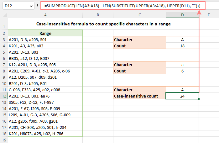
In the character of interest is input in a predefined cell, UPPER or LOWER will work equally well:
=SUMPRODUCT(LEN(A3:A18) - LEN(SUBSTITUTE(UPPER(A3:A18), UPPER(D2), "")))
Or
=SUMPRODUCT(LEN(A3:A18) - LEN(SUBSTITUTE(LOWER(A3:A18), LOWER(D2), "")))
The below screenshot shows it in action:
How to count certain text / substring in a range
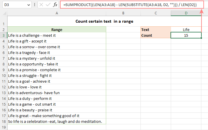
To count the number of occurrences of certain text in a range, use this generic formula:
For example, to count the number of times the word "Life" appears in the range A3:A18, the formula is:
=SUMPRODUCT((LEN(A3:A18) - LEN(SUBSTITUTE(A3:A18, D2, ""))) / LEN(D2))
Excel character limits for cells
Microsoft Excel has a limitation on the number of characters that can be entered in a cell. If you have worksheets with large amount of text data, you may find the following information helpful.
- The total number of characters that a cell can contain is 32,767.
- A cell can only display 1,024 characters. At the same time, the Formula bar can show all 32,767 symbols.
- The maximum length of a formula is 8,192 characters in Excel 2007 and higher (1,014 in Excel 2003).
Please consider the facts when you are going to merge or import data from an external source.
These are the best practices for counting characters in Excel. For first-hand experience, you can download a sample workbook and check out a list of related resources at the end of the page. Thank you for reading and hope to see you soon!
Practice workbook for download
Count characters in Excel - formula examples (.xlsx file)
 by
by
141 comments
How would I count the no of characters to the letter x
Eg 123x546789= 6
Hi! If I understand the question correctly, you can split a text string into individual characters using the MID function. Then you can use the MATCH function to find the position number of the character that you need to find.
=MATCH("x",MID(A1,ROW(A1:A20),1),0)
To find the number of characters before:
=MATCH("x",MID(A1,ROW(A1:A20),1),0)-1
To find the number of characters after:
=LEN(A1)-MATCH("x",MID(A1,ROW(A1:A20),1),0)
LEN function calculates the length of a text string.
BARB0JESALM --> HOW TO FIND 4 CHAR IS NUMBER OR TEXT IN EXCEL
Please clarify your specific problem or provide additional details to highlight exactly what you need. Maybe this article will be helpful: Excel substring: how to extract text from cell.
Hello,
You state;
”A cell can only display 1,024 characters. At the same time, the Formula bar can show all 32,767 symbols.”
This is not correct and applies only to Excel 2003 (and older). Starting with Excel 2007 all 32,767 characters allowed in a cell will be displayed correctly on the worksheet.
I'm wondering how to count the number of characters for each word in a sentence. For example:
A sentence in a single cell: I have a dog.
Would return: 1 4 1 4
I = 1
have = 4
a = 1
dog. = 4
Hello!
Split words into individual cells using one of these instructions: Split string by delimiter or pattern, separate text and numbers or TEXTSPLIT function in Excel: split text strings by delimiter. Then count the number of characters in each cell as described in the article above.
Hi. This is a long shot, but I have 180 rows of data that I'm having to print, then work out by hand the splits, then having to type them back into a grid.
They are 18 columns along, each with a letter which can be anything from A to Z.
They would read like this:
FFFFFFBICEDHFAPOPF
FAOPAPHDECIBFFFFFF
I'm trying to work out how to determine how many letters of the same value there are before the next letter.
There could be anything from 18 individual letters to 18 all of the same letter, so that:
FFFFFFBICEDHFAPOPF becomes 6F, 1B, 1I, 1C, 1E, 1D, 1H, 1F, 1A, 1P, 1O, 1P, 1F (because there are 6 Fs, then 1 B, then 1 I, etc)
and
FAOPAPHDECIBFFFFFF becomes 1F, 1A, 1O, 1P, 1A, 1P, 1H, 1D, 1E, 1C, 1I, 1B, 6F
They are each in individual columns at the moment, but I can CONCATENATE them if that's easier to determine it.
Thanks in advance.
To count a number of items (say each one represent machine number) in the follow
1,2,45,75,22,105,85
= count(textsplit(a2,",")
Hi!
I'm currently using a dropdown list to force a choice of 7 options 1, x , 2, 1x, x2, 12, 1x2.
And to get the most choosen value I've used: =INDEX(I2:N2;MODE(IF(I2:N2"";MATCH(I2:N2;I2:N2;0)))).
But the thing is it is counting 1x as one result, but I would rather it counted it as 1 "1" and one "x"
so for example if two people made their choices and chose 1x and 1, the above formula would show "1x" (as it is a tie but it is first in the column). I would like it to show 1 (count it as two number 1, and one X) instead. Is this possible?
Hello!
If I got you right, the formula below will help you with your task:
=INDEX(MID(CONCAT(I2:N2),ROW(1:20),1), MODE(IF(MID(CONCAT(I2:N2),ROW(1:20),1)<>"", MATCH(MID(CONCAT(I2:N2),ROW(1:20),1), MID(CONCAT(I2:N2), ROW(1:20),1),0))))
Hi again,
This was exactly what I was looking for, works like a charm!
Thanks a bunch!
Hi Again!
Is it possible to as well (in another cell) get the 2nd most chosen value?
I tried to get it through the below formula:
=INDEX(MID(CONCAT(I2:N2);ROW(1:20);1); MODE(IF(MID(CONCAT(I2:N2);ROW(1:20);1)"")*(MID(CONCAT(I2:N2);ROW(1:20);1);INDEX(MID(CONCAT(I2:N2);ROW(1:20);1);MODE(IF(MID(CONCAT(I2:N2);ROW(1:20);1)"";MATCH(MID(CONCAT(I2:N2);ROW(1:20);1);MID(CONCAT(I2:N2); ROW(1:20);1);0))))
But I'm definitely doing something wrong, and I realized I'm a bit above my knowledge level now as I don't fully comprehend the formula you helped me with (It works great though).
What I'm trying to achieve when it all is finished is one cell showing the most common value (as you helped me with above) and one cell showing the 2nd most common value and the difference between them, say If i have 5 "1" and 3 "x", The main goal is to get one (preferable) or two cells showing "X 2" as 5 - 3 = 2 (the difference).
I'm trying to read up on the above functions, but so far I'm not even sure if it is possible to do like I intended.
Hi!
I'm really sorry, we cannot help you with this task.
I am trying to exclude certain words/Text from the Filter. How do I uniquely count a column but ignore one repetitive entry.
I should add, this is similar to ignoring spaces etc. I want to ignore a word, using COUNTA(UNIQUE(FILTER( ))
Hello!
Use the SUMIFS function to calculate the sum of a column based on conditions. Here is a guide with examples: Excel SUMIFS and SUMIF with multiple criteria.
Hello
I am trying to get the bifurcation of categories of students in excel. but I can't get the result using the exists formulas in excel. Kindly help me to get it resolved.
The Problem is: In an attendance book there are 3 categories of students. the name of category is clearly mentioned in front of the name of the students. If there are 50 students in a classroom few students are belong to SC category, few are ST category and rest are General category. The attendance is marked P as present and A as Absent. Based on their categories, I have to calculate, how many SC category students are presented and in the same way other two categories.
Hi!
If you want to count values by two criteria, then use the COUNTIFS function.
An example formula for your data is
=COUNTIFS(A1:A10,"ST",C1:C10,"P")
Can anyone help me to get a group of frequency of "T" in the row as shown below using the excel formula? The frequency of "T" is 13 and the group of frequency of "T" is 5 (a set of T in a sequence is repeated 5 times). I need an excel formula to get 5.
O T T T O O T F F T T T O O V V F T T F F F O O O O O O T T T T
Hi!
Sorry, it's not quite clear what you are trying to achieve.
Hi,
I am using EXCEL 2007(IF FORMULA APPLICABLE IN LATEST VERSIONS OF EXCEL I CAN SWIFT TO NEW VERSIONS)
i need in a following data of some persons, if in case they are continuously "P", then at 7th place i have to note as "PW"
DAYS
SNO NAMES 1 2 3 4 5 6 7 8 9 10 11 12 13 14 15 16 17 18 19 20 21 22 23 24 25 26 27 28 29 30
1 JACK P P P P P P P P A P P P P P A P P P P P P P P P P P P P A A A P P P P P P P P P
2 JILL P P P P A A P P P P P P P P P P P P P A P P P P P P P P P P P P P P P A P P P P
3 JOHN P P P P P P P A A P P P A P A P P P P P P P P P P P P P A P P P P P A P P P P P
AFTER applying formula i want to get like this
1 JACK P P P P P P PW P A P P P P P P A P P P P P P PW P P P P P P A A A P P P P P P PW P P
2 JILL P P P P A A P P P P P P PW P P P P P P A P P P P P P PW P P P P P P PW P A P P P P
3 JOHN P P P P P P PW A A P P P A P A P P P P P P PW P P P P P P A P P P P P A P P P P P
KINDLY SHARE FORMULA to my mail id IF AVAILABLE(saisandeepnagari@hotmail.com), BY MANUALLY CHECKING AND TYPING, TIME TAKING PROCESS FOR LARGE DATA IN EXCEL
Hi!
If each line is text, then you can use the SUBSTITUTE function to find and replace characters.
=SUBSTITUTE(A2,"P P P P P P P","P P P P P P PW")
If each character is written in a separate cell, then you can only replace characters using a VBA macro.
Dear Sir,
Each P is written in separate Cell,
Kindly explain how to replace characters in VBA macro.
KINDLY SHARE FORMULA to my mail id IF AVAILABLE(saisandeepnagari@hotmail.com)
Hi!
You can concatenate separate cells into one string, as described in this guide: TEXTJOIN function in Excel - easy way to merge text from multiple cells.
For example,
=TEXTJOIN(" ",FALSE,A1:H1)
Then use the formula recommended for you to replace the characters. Then split the text into cells again. Read detailed instructions here: How to split cells in Excel: Text to Columns, Flash Fill and formulas.
Please please help me out of this
I want my work to look like this in 1 row (not in separate cells) Continuously :
"APPLE(5) BALL(4) CAT(3) DOG(3) ELEPHANT(8)"
Please help me out with a formula or an option.
Hi ,
I am having and issues where in row A i have 1234 and at row 100 i have 2314.
like that i have few number which is in permutation level.
The question is how to find out these number which is repeated as permutation .
Hello,
I have a work schedule, names on the left, days of the month on top. After placing an X for each persons name on the schedule I'm looking now for formulas that will see that X and then populate that persons name elsewhere on the sheet creating a daily roster of names that someone can easily copy down. Please help.
I want to count the letter of alpha numeric how many times itbwaa repeated in the sheet. Can you provide the answer.
Ex :
column a, row 1 : 1a,3b,2c
Column a, row 2 : 2a,3b,5d
Means here if if we use formula means when we search for 3b means the count should be 2.
Can you suggest how to write the code.
Hello!
Count the number of occurrences of certain text in a range - read above
Thanks for the reply,
I tried with same code in open office but it's not working it's showing #value instead of result. Is there any conflicts with "," in the column when we are searching with the formula which you gave. Actually my query is to find the alphanumeric ex : 2a how many times it's repeated along with another alphanumeric from column a row 1 to row 6
1a,2a,3a,5d
2c,4d,2a,7b
2a
3c,5d,6c
8a,11b
2a,10b
Now I want to search the letter 2a how many times repeated and it should be count even we are having "," in a cell.
My answer it should be 4 when we search from column A1:A6, similarly if we search for another alphanumeric also I need to get the result.
Hello!
Please try the following formula:
=SUM(--(ISNUMBER(FIND("2a",A1:A6,1))))
Ok I will and I will let u know.
Tried with the formula which you gave but not getting.
Is there any other formula...
Condition Report Type Sale
Condition 01 Sales Report 14
Condition 02 My Report 43
Condition 03 Report 25
Condition 04 Sales 76
Condition 05 Report 35
Condition 06 James's Report 85
Condition 07 Total 11
Condition 08 Report From my Boss 8
Condition 09 Not a Report 43
Count how many times words end with letter RT and contains 6 letters in Column C.
Hello Gajanan!
If I got you right, the formula below will help you with your task:
=SUM(--(RIGHT(C1:C10,2)="RT"))
=SUM(--(LEN(C1:C10)=6))
I hope it’ll be helpful.
how i count "p" in row in work sheet
Hi!
Change the formula that is recommended in this article
=SUM(LEN(A1:N1)-LEN(SUBSTITUTE(A1:N1,"p","")))
if i type in a cell 1 to 5 can i get total count
for example i type 77 to 80 can i got 2 count between 77 and 80
or i got 4 count between 77 and 80 when i include 77 and 80.
Please Help about Eg:-i want to calculate the Column B if in column A have "Y" Character
A B C D
1 X 2
2 Y 1
3 Z 3
4 Y 4
123456789 text box no how to count plz tell me formula
result 45 how
Thanks a ton for sharing this good info. If I can suggest, I'm likely not alone in finding the "Ultimate Suite" Ad with a scrolling gif hugely distracting. Someone obviously realized this and added a minimize function. Sadly, they only made the scrolling slightly smaller. This is why people use ad-blockers folks! :|
HI,
Going through you note helped me with working on a date wise schedule that spread across multiple rows which contained different programmes that are being aired. In this I had multiple advertisements placed which represented different product coded as A B and C etc. In come columns I had AD, and CA or any other combinations. As such i wanted to calculate all occurrences, and then create a summary of each representation.
This note simply helped with solving my problem.
Thank you and keep it up.
Sir,
Can excel show alphabet letter in against running number. Please explain formula.
For example, for value (.001 to .999 = A)
(1.00 to 1.99 = B)
(2.00 to 2.999= C).
Thanks!
Greetings
I am using this formula SUM(LEN(D21:D609)-LEN(SUBSTITUTE(D21:D609,"T","")))/LEN("T") as an array formula to count tears "T" recorded also using the same formula to count other quality faults such as bures "B"
I now wish to record the time taken to repair the tear or bure in column D21:D609 by entering T14B15 effectively the tear took 14 minutes to repair and the Bure took 15 minutes to repair what must I do to count total tears and sum the total minutes to repair the tear or the Bure?
Can you assist please
7411PG36353535 / 7411PG36353537 / 7411PG36353540 / 7411PG36353548 / 7411PG36354040 / 7411PG36354044 / 7411PG36354046 / 7411PG36354047 / 7411PG36354048 / 7411PG36355250 / 7411PG36355254 / 7411PG36355256 / 7411PG36357386
the above alphanumeric series in one cell, if i have to count the alphanumeric series then what formula i have to use
Hi,
I need a formula to pick 5 reviewed cases from their production irrespect of the production numbers.
Regards,
Ravi
How can I count an specific text that is marged with the few cells against a different column with the different texts.
For example in column A I have a name called "Backshell" or in other cell I have "Footwell"(but these names are marged in the multiple cells. Say Installation marged from A2 to A5 and Footwell from A6 to A10) and In column C I have many texts or words such as "Installation" or "Design" but the cells are not marged; I want to count how many times Installation has been repeated for just backshell or just Footwell.
Please help.
Thank you.
I have a problem that, i have different 100, 500 etc names
Problem: #01
i want to count duplicate name or same
Problem # 02:
Count its how much time in data
Problem # 03:
In same data reduced specific entry date wise
PLZ Help Me Anyone.......
Column Column Column
A B C
Karim 100 200
Rohim 200 300
Karim 100 500
Rohim 500 100
Result should be:
Karim 900
Rohim 1100
I used = sumproduct(Vlookup (A1,A1:C4,{2,3},0))
But it does not work. How can I do it? Pls help
Hi Guys,
I am not getting solve question that how will count this is.
please find below this question.
22pcs 5kg
15pcs 8kg
16pcs 10kg
65pcs 12kg
How will i count and sum please assist me.
Thanks and Regards,
Sujan
Sujan:
Enter "pcs" and "kg" in cells C62 and D62. These will be the headers.
Enter the data in A48:A57. The formula is case sensitive so be sure the data matches the caps in the headers.
In C63 enter =SUM(IF(ISNUMBER(FIND(C62,$A$48:$A$57)),VALUE(LEFT($A$48:$A$57,FIND(C62,$A$48:$A$57)-1)),0))
then with the cursor in the formula bar in the formula click the CTRL Shift Enter keys at the same time. This is an array formula so you need to tell Excel to evaluate it as an array. When you enter the formula and then in the formula bar you put the cursor in the formula and click the CTL SHIFT ENTER keys it will put curly brackets around the formula which indicates to Excel that this is an array.
When the value appears in C63 copy the formula over to D63.
As you enter more data in the A range be sure to change the second cell address to match the last cell in the range. Right now the range is A48 to A57. If you add more data change the A57 to another cell address. Remember, there are three places in the formula for that range.
Hi guys
i have query about this question how to spit number and text as like:- rana123ranjan456 and 1234sohan567raj how to use split number and text.
please assist me. please share this e-mail id abhisingh1111156@gmail.com
Thanks and Regards,
Sujan
Thanks Doug.
But is it possible to do sum without transferring text to the other column
I don't want the result like below:
20 cow
60 Cow
70 Cow
150
I want the result of sum like this:
20Cow
60Cow
70Cow
150Cow
Pls help how can I do.
Paul:
As is often the case in Excel, there are a couple of different ways to get to where you want to go.
Check out this article here on AbleBits for the explanations and examples of several ways to do what you're trying to do.
https://www.ablebits.com/office-addins-blog/excel-if-cell-contains-count-sum/
I want to do sum for the following which contain number & Words
20 cows
60 Cows
70 cows
Result should be 150 or 150 cows.
But if I use auto sum it does not work. How can I do it? Pls help me.
Paul:
Split the numbers from the words using Text-to-Columns.
Highlight the cell, go to Data then choose Text-to-Columns and follow the prompts. After the words and numbers have been separated into their own cells you can use =Sum on the cells that contain numbers.
sum samad26 karim26
how I will sum? please answer?
Hi,
I have data numeric and text with numeric, pls help here how could i count how many times 123456 in data sheet.
i hv use =SUMPRODUCT(--(LEFT(Sheet1!$G$2:$G$28069,6)=E4)) work ok, but when i was change formula =SUMPRODUCT(--((LEFT(Sheet1!G2:G28068,6)+0)=Sheet2!C3)) this was not working.
123456-1234
321654-3214
456789-8579
PO111991
123456-1234
Hello
How do i count a reply yes for example for cells not arranged within a range
E. G
I created a checklist on excel and the reply to the answers yes/no as per the questions are not arranged in typical range
Result analysis formular in excel
i want to make result analysis in a way i want the number of As,Bs, Cs etc
on a excel templete using formular.
Best Regards
NWANNA, D.
i want to convert "PP" into numeric in attendance sheet
example :- "P" count 1, if we insert double P into one Cell of MS Excel then count 2
I am trying to count the number of names in a cell. What formula would I use to do this? The name format is first and last which would count as one name.
Dear Natalia,
I would like to clarify...I have a attendence sheet..it cotains Present,Sick leave and annual leave...I use countif formula to get total sick leave and annual leave.then got data.
But when i filer the sheet based on user the total sick leave and annual leave are not changing.still showing same number...i am requsting to get a formula to solve this issue...
When filter sheet by name result should be show only filtered user only...subtotal formula
I hope clear my question...your quick reply highly appreciated
Hello,
For me to understand the problem better, please send me a small sample workbook with your source data and the result you expect to get to support@ablebits.com.
Please also don't forget to include the link to this comment into your email.
I'll look into your task and try to help.
How can use countif function in subtotal formula...
when i use subtotal function i couldnot find countif formula in the list...there is count and countA in the list...
thank you in advance for your valuable support