The tutorial will teach you how to find an average in Excel with or without formulas and round the results to as many decimal places as you want.
In Microsoft Excel there are a handful of different functions for calculating the average for a set of numeric values. Moreover, there is an instant non-formula way. On this page, you will find a quick overview of all the methods illustrated with examples of use and best practices. All the functions discussed in this tutorial work in any version of Excel 365 through Excel 2007.
What is average?
In everyday life, the average is a number expressing the typical value in a dataset of data. For example, if a few athletes have run a 100m sprint, you may want to know the average result - i.e. how much time most sprinters are expected to take to complete the race.
In mathematics, the average is the middle or central value in a set of numbers, which is calculated by dividing the sum of all the values by their number.
In the above example, assuming the first athlete covered the distance in 10.5 seconds, the second needed 10.7 seconds, and the third took 11.2 seconds, the average time would be 10.8 seconds:
(10.5+10.7+11.2)/3 = 10.8
How to get average in Excel without formulas
In Excel worksheets, you do not need to perform manual calculations - powerful Excel functions will do all the work behind the scenes and deliver the result in no time. Before exploring the specialized functions in detail, let's learn a quick and amazingly simple non-formula way.
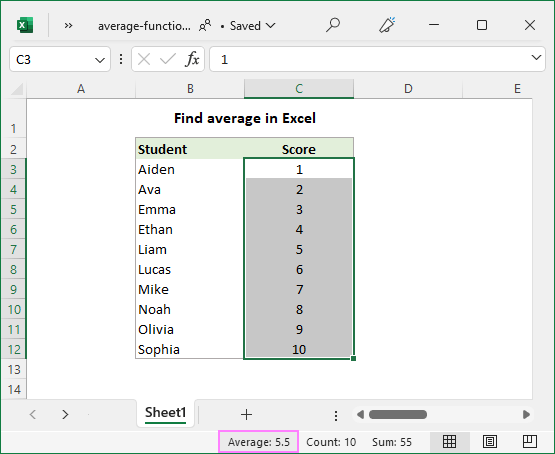
To quickly find an average without a formula, use Excel's status bar:
- Select the cells or ranges you want to average. For non-contiguous selections, use the Ctrl key.
- Look at the status bar at the bottom of the Excel window, which provides the essential information about the currently selected cells. One of the values that Excel calculates automatically is the average.
The result is shown in the image below:
If average is not displayed for your dataset, this article explains possible causes and solutions: Why Excel is not showing sum, average or count in the status bar.
How to calculate average manually
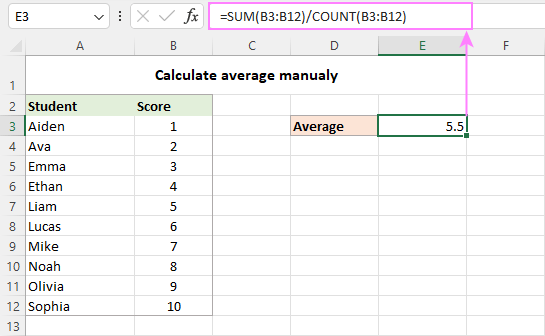
In math, to find the arithmetic mean of a list of numbers, you need to add up all the values, and then divide the sum by how many numbers there are in the list. In Excel, this can be done using the SUM and COUNT functions, respectively:
For the range of numbers below, the formula goes as follows:
=SUM(B3:B12)/COUNT(B3:B12)
As you can see, the result of the formula exactly matches the average value in the status bar.
In practice, you will hardly ever need to do a manual average in your worksheets. However, it may be useful to re-check the result of your average formula in case of doubt.
And now, let's take a look at how you can do average in Excel using the functions specially designed for the purpose.
AVERAGE function - calculate an average of numbers
You use the Excel AVERAGE function to get an average of all numbers in the specified cells or ranges.
Where number1, number2, … are numeric values for which you want to find the average. Up to 255 arguments can be included in a single formula. The arguments can be supplied as numbers, references, or named ranges.
AVERAGE is one of the most straightforward and easy-to-use functions in Excel.
To calculate an average of numbers, you can type them directly in a formula or supply the corresponding cell or range references.
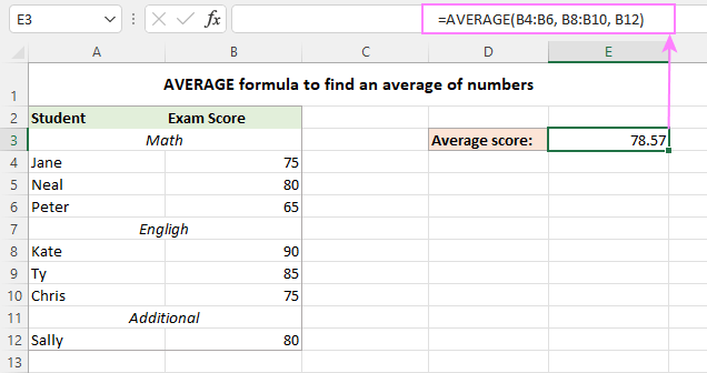
For example, to average 2 ranges and 1 individual cell below, the formula is:
=AVERAGE(B4:B6, B8:B10, B12)
Apart from numbers, the Excel AVERAGE function can find an average of other numeric values such as percentages and times.
Excel AVERAGE formula - usage notes
As you've just seen, using the AVERAGE function in Excel is easy. However, to get a correct result, you need to clearly understand what values are included in the average and what are ignored.
Included:
- Cells with zero values (0)
- Logical values TRUE and FALSE typed directly into the list of arguments. For example, the formula AVERAGE(TRUE, FALSE) returns 0.5, which is the mean of 1 and 0.
Ignored:
- Empty cells
- Text strings
- Cells containing Boolean values TRUE and FALSE
For more information, please see How to use AVERAGE function in Excel.
AVERAGEA function - average all non-blank cells
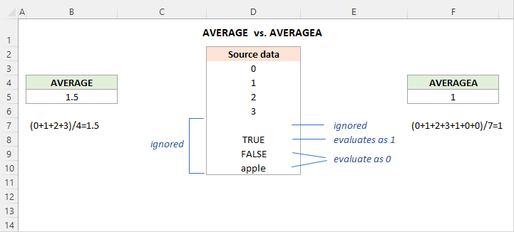
The Excel AVERAGEA function is similar to AVERAGE in that it calculates the arithmetic mean of the values in its arguments. The difference is that AVERAGEA includes all non-empty cells in a calculation, whether they contain numbers, text, logical values, or empty strings returned by other functions.
Where value1, value2, … are values, arrays, cell references or ranges that you want to average. The first argument is required, others (up to 255) are optional.
Excel AVERAGEA formula - usage notes
As mentioned above, the AVERAGEA function processes different value types such as numbers, text strings and logical values. And here's how they are evaluated:
Included:
- Text values evaluate as 0.
- Zero-length strings ("") evaluate as 0.
- Boolean value TRUE evaluates as 1 and FALSE as 0.
Ignored:
- Empty cells
For example, the below formula returns 1, which is the average of 2 and 0.
=AVERAGEA(2, FALSE)
The following formula returns 1.5, which is the average of 2 and 1.
=AVERAGEA(2, TRUE)
The image below demonstrates the AVERAGE and AVERAGEA formulas applied to the same list of values and different results they return:
AVERAGEIF function - get average with condition
To get the average of all cells in the specified range that meet a certain condition, use the AVERAGEIF function.
The AVERAGEIF function has the following arguments:
- Range (required) - the range of cells to test against a given criteria.
- Criteria (required) - the condition that should be met.
- Average_range (optional) - the cells to average. If omitted, then range is averaged.
The AVERAGEIF function is available in Excel 2007 - Excel 365. In earlier versions, you can build your own AVERAGE IF formula.
And now, let's see how you can use the Excel AVERAGEIF function to average cells based on the condition you specify.
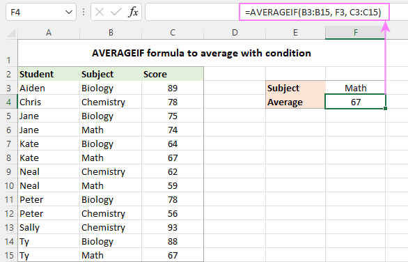
Suppose you have scores for different subjects in C3:C15 and you wish to find an average math score. This can be done with the following formula:
=AVERAGEIF(B3:B15, "math", C3:C15)
Instead of "hardcoding" the condition directly in a formula, you can type it in a separate cell (F3) and refer to that cell in the criteria:
=AVERAGEIF(B3:B15, F3, C3:C15)
For more formula examples, please see Excel AVERAGEIF function.
AVERAGEIFS function - average with multiple criteria
To do average with two or more conditions, use the plural counterpart of AVERAGEIF - the AVERAGEIFS function.
The function has the following syntax:
- Average_range (required) - the range to average.
- Criteria_range (required) - the range to be tested against criteria.
- Criteria (required) - the condition that determines which cells to average. It can be supplied in the form of a number, logical expression, text value, or cell reference.
1 to 127 criteria_range / criteria pairs can be supplied. The first pair is required, subsequent ones are optional.
In essence, you use AVERAGEIFS similarly to AVERAGEIF, except that more than one condition can be tested within a single formula.
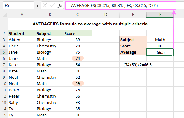
Supposing some students did not take tests in certain subjects and have zero scores. You aim to find an average score in a specific subject ignoring zeros.
To accomplish the task, you build an AVERAGEIFS formula with two criteria:
- Define the range to average (C3:C15).
- Specify the range to check against the 1st condition (B3:B15 - items).
- Express the 1st condition ("math" or F3 - the target item enclosed in quotation marks or reference to the cell containing the item).
- Specify the range to check against the 2nd condition (C3:C15 - scores).
- Express the 2nd condition (">0" - greater than zero).
By assembling the above components together, we get the following formula:
=AVERAGEIFS(C3:C15, B3:B15, "math", C3:C15, ">0")
Or
=AVERAGEIFS(C3:C15, B3:B15, F3, C3:C15, ">0")
The image below makes it clear that only two cells (C6 and C10) meet both conditions, and therefore only these cells are averaged.
For more information, check out Excel AVERAGEIFS function.
AVERAGEIF and AVERAGEIFS formulas - usage notes
Excel AVERAGEIF and AVERAGEIFS functions have much in common, in particular which values they calculate and which ignore:
- In the average range, empty cells, text values, logical values TRUE/FALSE are ignored.
- In criteria, empty cells are treated as zero values.
- The wildcard characters such as question mark (?) and asterisk (*) can be used in criteria for partial match.
- If no cell meets all of the specified criteria, a #DIV0! error occurs.
AVERAGEIF vs. AVERAGEIFS - differences
In terms of functionality, the most essential difference is that AVERAGEIF can only handle one condition while AVERAGEIFS one or more criteria. Also, there are a couple of technical differences related to average_range.
- With AVERAGEIF, average_range is the last and optional argument. In AVERAGEIFS formulas, it is the first and required argument.
- With AVERAGEIF, average_range does not necessarily have to be the same size as range because the actual cells to be averaged are determined by the size of the range argument - the upper left cell of average_range is taken as the starting point, and as many cells are averaged as included in the range argument. AVERAGEIFS requires each criteria_range to be of the same size and shape as average_range, otherwise a #VALUE! error occurs.
AVERAGE IF OR formula in Excel
Since the Excel AVERAGEIFS function always works with the AND logic (all criteria must be TRUE), you will have to construct your own formula to average cells with the OR logic (any single criterion must be TRUE).
Here's the generic formula to average if cell is X or Y.
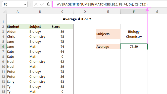
Now, let's see how it works in practice. In the table below, suppose you want to find an average score of two subjects, Biology and Chemistry, which are input in cells F3 and F4. This can be done with the following array formula:
=AVERAGE(IF(ISNUMBER(MATCH(B3:B15, {"biology", "chemistry"}, 0)), C3:C15))
Translated into a human language, the formula says: average cells in C3:C15 if a corresponding cell in B3:B15 is either "Biology" or "Chemistry".
Instead of the hardcoded criteria, you can use a range reference (F3:F4 in our case):
=AVERAGE(IF(ISNUMBER(MATCH(B3:B15, F3:F4, 0)), C3:C15))
For the formula to work correctly, please remember to press Ctrl + Shift + Enter in Excel 2019 and lower. In dynamic array Excel (365 and 2021), a regular Enter hit will suffice:
How this formula works:
For our curious and thoughtful readers who want not only to use a formula but understand what they are doing, here's a detailed explanation of the logic.
At the core of the formula, the IF function determines which values in the source range match any of the specified criteria and passes those values to the AVERAGE function. Here's how:
The MATCH function uses the subject names in B3:B15 as the lookup values and compares each of those values against the lookup array in F3:F4 (our target subjects). The 3rd argument (match_type) is set to 0 to look for exact match:
MATCH(B3:B15, F3:F4, 0)
When a match is found, MATCH returns its relative position in the lookup array, otherwise an #N/A error:
{1;2;1;#N/A;1;#N/A;2;#N/A;1;2;2;1;#N/A}
The ISNUMBER function converts numbers to TRUE and errors to FALSE:
{TRUE;TRUE;TRUE;FALSE;TRUE;FALSE;TRUE;FALSE;TRUE;TRUE;TRUE;TRUE;FALSE}
This array goes to the logical test of IF. In the full form, the logical test should be written like this:
IF(ISNUMBER(MATCH(B3:B15, F3:F4, 0))=TRUE
For the sake of brevity, we omit the =TRUE part because it's implied.
By setting the value_if_true argument to C3:C15, you tell the IF function to replace TRUE's with the actual values from C3:C15:
{89;78;75;FALSE;64;FALSE;62;FALSE;78;56;93;88;FALSE}
This final array is handed over to the AVERAGE function that calculates an arithmetic mean of numbers ignoring logical values.
How to round average in Excel
When calculating an average in Excel, the result is often a number with multiple decimal places. In case you want to display fewer decimal digits or round an average to an integer, use one of the following solutions.
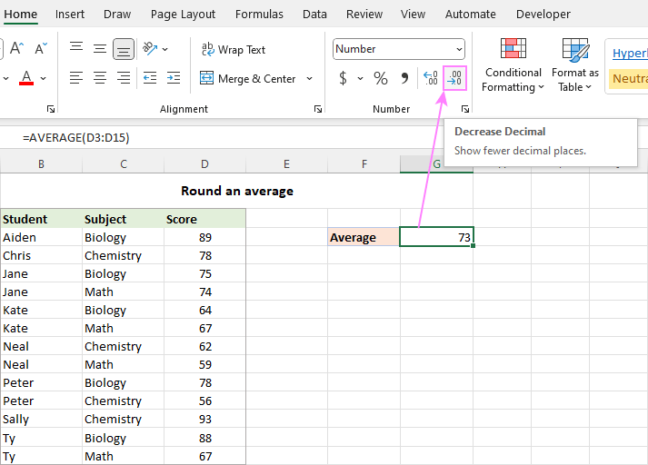
Decrease Decimal option
To round only the displayed average without changing the underlying value, the fastest way is to utilize the Decrease Decimal command on the Home tab, in the Number group:
Format Cells dialog box
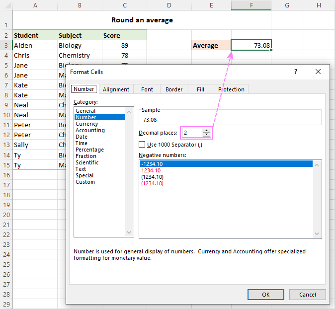
The number of decimal places can also be specified in the Format Cells dialog box. To have it done, select the formula cell and press Ctrl + 1 to open the Format Cells dialog. Then, switch to the Number tab, and type the number of places you want to show in the Decimal places box.
Like the previous method, this changes only the display format. When referring to the average cell in other formulas, the original non-rounded value will be used in all calculations.
For full details, please see Round numbers by changing cell format.
Round an average with a formula
To round the calculated value itself, wrap your average formula in one of the Excel rounding functions.
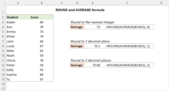
In most situations, you'd use the ROUND function that follows the general math rules for rounding. In the 1st argument (number), nest the AVERAGE, AVERAGEIF or AVERAGEIFS function. In the 2nd argument (num_digits), specify the number of decimal places to round the average to.
For example, to round off an average to the nearest integer, the formula is:
=ROUND(AVERAGE(B3:B15), 0)
To round an average to one decimal place, this is the formula to use:
=ROUND(AVERAGE(B3:B15), 1)
To round an average to two decimal places, this one will work:
=ROUND(AVERAGE(B3:B15), 2)
That is how you can do average in Excel. Below there are links to the related tutorials that discuss more specific cases of average, hope you will find them helpful. Thank you for reading!
Practice workbook for download
Calculate average in Excel - examples (.xlsx file)
 by
by
105 comments
Thank you for our column.
my question is I want the average temperature for the past 10 days.
The temperatures are in column A rows 2 through 11
The average is calculated in Column B Row 1
On day 11 I want to add the current temperature, preferably in Column A row 2 using INSERT and moving the old data down 1 row.
Using a $ to designate absolute cells does not work, when I use INSERT the formula changes to match the old data.
For example before insert the formula is: =Average(A$2:A$11 but after inserting a cell in A2 and selecting "shift cells down" the formula changes to =Average(A$3:A$12)
Thank you for any assistance
Hello! Convert the range A1:A11 into a table. Read how to do it here: Excel table: end-to-end tutorial with examples. Use structured references in the formula for calculating the average value. For example:
=AVERAGE(Table1[temp])
Then when you insert row 2, a row will be added to the table and the formula will not change.
Thank you very much for your assistance!
Hi, I'm trying to get the averages of stats after each basketball game in a season; i.e., free throws, rebounds, etc. I have manually entered the first four 'average' formulas, but wanted to have it done automatically with a formula, so i didn't have to add each new game to the formula manually. Here is a portion of my spreadsheet:
Rebounds Avg Rebounds
3 3
6 4.5
3 4
4 * this column is where I want the formula to automatically calculate so I don't have to manually update the formula after every game
Hi! Maybe this article will be helpful: How to copy formula in Excel with or without changing references.
Hi, how can write the average of a set of numbers up to the present month , excluding the on coming months?
For example the present month is October:
Month Numbers
Jan. 12
Feb. 20
Mar. 5
Apr. 45
May 60
Jun. 3
Jul. 12
Aug. 25
Sept. 7
Oct. 4
Nov. 0
Dic. 0
Hi! I don't quite understand what value you want to get. But you can calculate the average value by conditions using the AVERAGEIFS function. Look for the example formulas here: Excel AVERAGEIFS function with multiple criteria. I hope it’ll be helpful. If this is not what you wanted, please describe the problem in more detail.
Hi,
in excel, while taking the average of two components, if one component is 0 (zero) and second component shall be reported as result.
How can I make a formula for this in excel.
Thanks in advance.
Hi! Use the AVERAGE function for the two cells as recommended in the article above.
1st month revenue 15 Rs 18Th Month Total revenue is 188 Rs .But How can we chek avg revenue middle of the months
You can calculate the average value using the AVERAGE function as described in the article above.
Can I use AVERAGEIFS to get the average of two AVERAGEIFS calculations?
Example: I want to calculate the average of both of these ranges located on two separate sheets
=averageifs('2022 Survey Data'!D:D, '2022 Survey Data'!L:L, ">04/01/2022",'2022 Survey Data'!L:L,"<05/01/2022", '2022 Survey Data'!D:D, "")
and
=averageifs('2022 Zoom Data'!D:D, '2022 Zoom Data'!L:L, ">04/01/2022",'2022 Zoom Data'!L:L,"<05/01/2022", '2022 Zoom Data'!D:D, "")
Hello!
I can't check the formula that contains unique references to your workbook worksheets. Each of your formulas returns a value to the cell in which it is written. Calculate the average of these two cells using the AVERAGE function.
Or you can use these formulas as arguments for the AVERAGE function.
=AVERAGE(averageifs(‘2022 Survey Data’!D:D, ‘2022 Survey Data’!L:L, “>04/01/2022″,’2022 Survey Data’!L:L,”<05/01/2022", '2022 Survey Data'!D:D, "”), averageifs(‘2022 Zoom Data’!D:D, ‘2022 Zoom Data’!L:L, “>04/01/2022″,’2022 Zoom Data’!L:L,”<05/01/2022", '2022 Zoom Data'!D:D, "”))
What is the excel formula for calculating the value of the simple average in the candlestick chart for stock trading, as the period changes from one to two days.
Dear Svetlana
I need to easy average fonction. I have table for sold products KG and the rate. I need to average rate of the each products. You can see below a small table but my real table is huge.
Product - KG - Rate
A - 120 - 1,50
B - 85 - 3,40
C - 90 - 2,75
A - 110 - 1,53
A - 113 - 1,48
C - 85 - 2,68
Hello!
If you want to calculate the average for a product, use the AVERAGEIF function as described in this article. If you need to calculate a weighted average, use this guide.
Hi, fab article. Is there any way to do an AverageIF on selected cells within a row. E.g. the data to average is not continuous but has gaps to avoid?
Many thanks
Hi,
If by gaps you mean empty cells, then this case is described in detail in the manual above. Use AVERAGEIFS. Also remember that there can only be one counting range for the AVERAGEIF function.
date day hour time temp hour
1/1/12 0:00 1 1 0 0:00 10.7 day 0 1 2 3.........24
1/1/12 0:05 1 1 0 0:05 10.8 1 27.6
1/1/12 0:10 1 1 0 0:10 11 2
1/1/12 0:15 1 1 0 0:15 11.2 3
1/1/12 0:20 1 1 0 0:20 11 4
1/1/12 0:25 1 1 0 0:25 10.8 5
1/1/12 0:30 1 1 0 0:30 10.9 6
1/1/12 0:35 1 1 0 0:35 10.8 7
1/1/12 0:40 1 1 0 0:40 10.6 8
1/1/12 0:45 1 1 0 0:45 10.6 9
1/1/12 0:50 1 1 0 0:50 10.9 10
1/1/12 0:55 1 1 0 0:55 10.8 11
1/1/12 1:00 1 1 1 1:00 10.8 12
1/1/12 1:05 1 1 1 1:05 10.7 13
1/1/12 1:10 1 1 1 1:10 10.5 14
1/1/12 1:15 1 1 1 1:15 10.6 366
my data is a 5-minutes interval data for the year 2012, i want to get hourly average for each day of the 366days, the complete data has 105408 points, my AVERAGEIFS gives me 27.6 instead of 10.8, the code below is what i used and my excel version is 2007.
=AVERAGEIFS($G$2:$G$105409, $C$2:$C$105409, $L3,$D$2:$D$105409,M$2)
warm regards
Chris
Hello!
Based on your description, it is hard to completely understand your task.
What result do you want to get? Are you looking for 366 daily average temperatures? Or do you want averages for each hour?
However, I’ll try to guess: if column G is temperature, C is date, D is the ordinal number of the hour (0, 1 ....), then your formula will determine the average temperature value for any hour of any date.
You can get the ordinal number of the hour using the HOUR([time]) function.
I need to average every 5th cell in a row for a workbook that will be recording daily input, it needs to extend on for continued use. I'm using this format and from what I can tell it should work, but averages are puling numbers from every cell not just every 5th cell.
=Average(IF(MOD(COLUMN(G3:AA3),5)=0,G3:AA3))
Yes, I am pressing Shift+Ctrl+Enter.
Please Help
Lol, guess i should have checks to see if anyone was answering all the questions before I asked mine.
Hello!
If I understand your task correctly, the following formula should work for you:
=Average(IF(MOD(COLUMN(G3:AA3),5)=1,G3:AA3))
I hope it’ll be helpful.
I need a formula to help find the average time between repeat customers. For example, I have the date the customer placed the order in column A, I have the customers name in column B. How do I find the average date between when a customers name is repeated
I need an excel formula to find daily average of data taken multiple times daily for 10years. What formula will work for me
Hi,
I have a worksheet with many columns right beside each other, and two of the cells in each column that are vertical from one another need to be averaged independently. The two cells in each column that are averaged are dates. I used the formula =AVERAGE(27:27),27:27 is where both dates are placed, but after I pasted my second column beside the first, the second columns average date was affected by the first two dates in the firs column. I guess I told the formula to average ALL the dates together. I want each column to average it's own dates separate without being affected by the other columns. Is there a way to do this? I will be adding a lot more columns in the future so I need a formula that's short. Thanks.
Hi,
I am trying to have AVERAGE of a column with AVERAGEIFS option. It gives me error with below formula. It gives error after use "0" at the end of formula too.
What could be the right one.
Thanks in advance.
=AVERAGEIFS(ALL!J:J;ALL!$D:$D;D5;ALL!$G:$G;$I$4)
I am trying to average between a set range. I want to exclude anything below 10 and over 70.
Example
50
8
6
40
80
The average I want to get is 45 but cant find a formula to do this. Please help.
Is there a formula in MS-Excel 2016 that can provide an average if every other cell is a percentage? Only want the averages of the percentages for a specific cell range
I want to perform all the calculations in one cel,item,Quantity and Moisture weighted average in exal
Hello,
I need your help, one excel in this formula use, after use this formula i am unable to use this formula.
=IF(F7<1,"87",IF(F7<2,"85",IF(F7<3,"82",IF(F7<4,"82",IF(F7<5,"78",IF(F7<6,"75",IF(F7<7,"72")))))))
Please help
I am working working on data in 2 sheets with similar dimensions.
The data is for many countries, and stretches over 22 years.
Sheet 1 categorises data into 3 codes: 0, 1, 2 (0=not traded at all; 1=traded at begining; and 2=not traded in the last 2 years)
Sheet 2 contains values values (exports) corresponding to cartegories 0, 1 and 2.
Now, I would like to find average values for each cartegory. In other words I am trying to find the average for Cartegory 0; Cartegory 1 and Cartegory 3. How do I find the average.
I appreciate your help.
Thank you.
I've got an averages calculation with every other non-adjacent cell
=AVERAGE(B5,D5,F5) etc currently up to SN5 which is 255 numbers. When I try to add the next one in, I keep getting "You've entered too many arguments for this function" but there are no arguments, it's just an average. I've checked to make sure there are no cells in the calculation that shouldn't be there, and everything looks as it should be. Is there a maximum on the number of data cells in an averages calculation? Surely not? Please help!!
Hi!
I have a daily work in regards with excel, we had an instruction that goes like this "If the sale of this person is below the average of everyone, the commission must be 5%, and 10% if above the average all.
In the column, the result must be either 5% or 10%." I really am having a hard time using the right formula.
Hoping for your positive response.
Thank you!