This short tutorial explains the basics of the Excel COUNT and COUNTA functions and shows a few examples of using a count formula in Excel. You will also learn how to use the COUNTIF and COUNTIFS functions to count cells that meet one or more criteria.
As everyone knows, Excel is all about storing and crunching numbers. However, apart from calculating values, you may also need to count cells with values - with any value, or with specific value types. For example, you may want a quick count of all items in a list, or the total of inventory numbers in a selected range.
Microsoft Excel provides a couple of special functions for counting cells: COUNT and COUNTA. Both all very straightforward and easy-to-use. So let's take a quick look at these essential functions first, and then I will show you a few Excel formulas to count cells that meet certain condition(s), and clue you in on the quirks in counting some value types.
Excel COUNT function - count cells with numbers
You use the COUNT function in Excel to count the number of cells that contain numerical values.
The syntax of the Excel COUNT function is as follows:
Where value1, value2, etc. are cell references or ranges within which you want to count cells with numbers.
In Excel 365 - 2007, the COUNT function accepts up to 255 arguments. In earlier Excel versions, you can supply up to 30 values.
For example, the following formula returns the total number of numeric cells in range A1:A100:
=COUNT(A1:A100)
Note. In the internal Excel system, dates are stored as serial numbers and therefore the Excel COUNT function counts dates and times as well.
Using COUNT function in Excel - things to remember
Below are the two simple rules by which the Excel COUNT function works.
- If an argument(s) of an Excel Count formula is a cell reference or range, only numbers, dates and times are counted. Blanks cells and cells containing anything but a numeric value are ignored.
- If you type values directly into the Excel COUNT arguments, the following values are counted: numbers, dates, times, Boolean values of TRUE and FALSE, and text representation of numbers (i.e. a number enclosed in quotation marks like "5").
For example, the following COUNT formula returns 4, because the following values are counted: 1, "2", 1/1/2016, and TRUE.
=COUNT(1, "apples", "2", 1/1/2016, TRUE)
Excel COUNT formula examples
And here are a few more examples of using the COUNT function in Excel on different values.
To count cells with numeric values in one range, use a simple count formula like
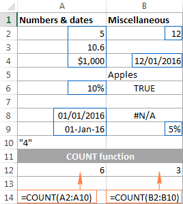
=COUNT(A2:A10)
The following screenshot demonstrates which types of data are counted and which are ignored:
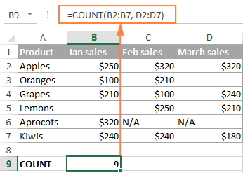
To count several non-contiguous ranges, supply all of them to your Excel COUNT formula. For example, to count cells with numbers in columns B and D, you can use formula similar to this:
=COUNT(B2:B7, D2:D7)
Tips:
Excel COUNTA function - count non-blank cells
The COUNTA function in Excel counts cells containing any value, i.e. cells that are not empty.
The syntax of the Excel COUNTA function is akin to that of COUNT:
Where value1, value2, etc. are cell references or ranges where you want to count non-blank cells.
For example, to count cells with value in range A1:A100, use the following formula:
=COUNTA(A1:A100)
To count non-empty cells in several non-adjacent ranges, use a COUNTA formula similar to this:
=COUNTA(B2:B10, D2:D20, E2:F10)
As you can see, the ranges supplied to an Excel COUNTA formula do not necessarily need to be of the same size, i.e. each range may contain a different number of rows and columns.
Please keep in mind that Excel's COUNTA function counts cells containing any type of data, including:
- Numbers
- Dates / times
- Text values
- Boolean values of TRUE and FALSE
- Error values like #VALUE or #N/A
- Empty text strings ("")
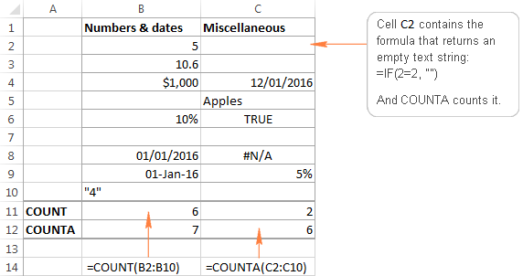
In some cases, you may be perplexed by the COUNTA function's result because it differs from what you see with your own eyes. The point is that an Excel COUNTA formula may count cells that visually look empty, but technically they are not. For example, if you accidentally type a space in a cell, that cell will be counted. Or, if a cell contains some formula that returns an empty string, that cell will be counted as well.
In other words, the only cells that the COUNTA function does not count are absolutely empty cells.
The following screenshot demonstrates the difference between Excel COUNT and COUNTA functions:
For more ways to count non-blank cells in Excel, check out this article.
Tip. If you just want a quick count of non-blank cells in a selected range, simply have a look at Status Bar at the bottom right corner of your Excel window:
![]()
Other ways to count cells in Excel
Aside from COUNT and COUNTA, Microsoft Excel provide a few other functions to count cells. Below you will discuss 3 most common use cases.
Count cells that meet one condition (COUNTIF)
The COUNTIF function is purposed for counting cells that meet a certain criterion. Its syntax requires 2 arguments, which are self-explanatory:
In the first argument, you define a range where you want to count cells. And in the second parameter, you specify a condition that should be met.
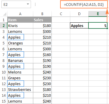
For example, to count how many cells in range A2:A15 are "Apples", you use the following COUNTIF formula:
=COUNTIF(A2:A15, "apples")
Instead if typing a criterion directly in the formula, you can input a cell reference as demonstrated in the following screenshot:
For more information, please see How to use COUNTIF in Excel.
Count cells that match several criteria (COUNTIFS)
The COUNTIFS function is similar to COUNTIF, but it allows specifying multiple ranges and multiple criteria. Its syntax is as follows:
The COUNTIFS function was introduced in Excel 2007 and is available in all later versions of Excel 2010 - 365.
For example, to count how many "Apples" (column A) have made $200 and more sales (column B), you use the following COUNTIFS formula:
=COUNTIFS(A2:A15,"apples", B2:B15,">=200")
To make your COUNTIFS formula more versatile, you can supply cell references as the criteria:
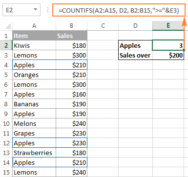
You will find plenty more formula examples here: Excel COUNTIFS function with multiple criteria.
Get a total of cells in a range
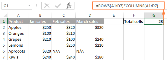
If you need to find out the total number of cells in a rectangular range, utilize the ROWS and COLUMNS functions, which return the number of rows and columns in an array, respectively:
=ROWS(range)*COLUMNS(range)
For example, to find out how many cells there are in a given range, say A1:D7, use the following formula:
=ROWS(A1:D7)*COLUMNS(A1:D7)
Well, this is how you use the Excel COUNT and COUNTA functions. Like I said, they are very straightforward and you are unlikely to run into any difficulty when using your count formula in Excel. If someone knows and is willing to share some interesting tips on to how to count cells in Excel, your comments will be greatly appreciated. I thank you for reading and hope to see you on our blog next week!
 by
by
113 comments
I want to know how to count male and female having specific degree. for eg. If I am preparing table for interview of teachers and applicants are male and female with qulifications like ph. d. m.sc. m.a. net or set etc. the how to calculate how many male are Phd or net or only m.sc. if we have written all their qualification in one row only.
Hi! Use SUMPRODUCT function to count values on multiple criteria.
The formula might look like this:
=SUMPRODUCT((A2:A20="male")*(ISNUMBER(SEARCH("m.sc",B2:B20))))
Also, take a look at this article : How to find substring in Excel
I'm wanting to add data after a counta formula. How/Can I do that? Example: Column A ...my formula is =counta(a2:a50) and that total is 49 ....I'm wanting to add the words Employees Shift A after it in the same cell. Can't figure out how to do that.
Any help would be greatly appreciated.
Thanks!!
Hi! Look for the example formulas here: Join text string and another function. This should solve your task.
30 parcels =1 person than 1000= ? person in excel rules.. please help to me
I need to your help with a formula im trying to build and its been days I have tried my ways but I haven’t reached anywhere
1. I filter the data by Month as I have 6 months data.
2. I filter it by unit as I have two unit
3. I have 8 different columns with 8 metrics.
4. 1st select the first data column and sort is desc to asc.
5. I count the total day on that column.
6. For eg if its 50 then I need the top 30. Mid 40 and bottom 30
7. I multiply 50*30% give me m top30 and bottom 30 which is 15 each
8. Remaining 20 as my mid40 percent
9. I have to do this manually and assign the name on E Column for the first 15 entries as T30 then go on to other 20 and type M40 and remaining as B30.
10. Now I have data in thousands and it’s a very tedious task to do this everytime manually.
Is tehre a way to create a formula which takes count and cover the cells I need to my to mid and bottow.
Month Center Unit Work per hour
May-22 Mumbai BC 100 T30
May-22 Mumbai BC 66 T30
May-22 Mumbai BC 64 T30
May-22 Mumbai BC 63 T30
May-22 Mumbai BC 56 T30
May-22 Mumbai BC 55 T30
May-22 Mumbai BC 46 T30
May-22 Mumbai BC 42 T30
May-22 Mumbai BC 41 T30
May-22 Mumbai BC 36 M40
May-22 Mumbai BC 30 M40
May-22 Mumbai BC 30 M40
May-22 Mumbai BC 29 M40
May-22 Mumbai BC 28 M40
May-22 Mumbai BC 27 M40
May-22 Mumbai BC 26 M40
May-22 Mumbai BC 25 M40
May-22 Mumbai BC 23 M40
May-22 Mumbai BC 23 M40
May-22 Mumbai BC 22 M40
May-22 Mumbai BC 20 M40
May-22 Mumbai BC 19 M40
May-22 Mumbai BC 18 M40
May-22 Mumbai BC 17 M40
May-22 Mumbai BC 14 B30
May-22 Mumbai BC 12 B30
May-22 Mumbai BC 11 B30
May-22 Mumbai BC 10 B30
May-22 Mumbai BC 9 B30
May-22 Mumbai BC 8 B30
May-22 Mumbai BC 6 B30
May-22 Mumbai BC 5 B30
May-22 Mumbai BC 1 B30
If I calculate rolls for example +70+50+70+70 of different yardings in one cell and i want to know the quantity of rolls (i.e., 4) in different cells. Then what formula should i apply?
Hi!
To count the number of numeric values, use these guidelines: Count if cell contains number.
Problem: "Formula where result on Sheet 2 is generated from data on sheet 1"
Hi,
I want to write a formula like (len(AO2)) to calculate string characters in a cell in sheet2 having data from sheet1. How it will be done?
How to combine COUNTIFS ADN COUNTA like this
=COUNTIFS(C$9:C$707,B717,Q$9:Q$707,COUNTA(Q$9:Q$707))
Hello!
Seeking kind assistance I have Record Sales Monitoring, how to count TR NO. in Excel?
Situation - I want to count Sales Transaction Number per Date?
Date TR NO . Subtotal
11/13/20 12344 95.50
11/15/20 12345 428.00
11/15/20 12345 398.00
11/16/20 12350 179.00
Hi,
To calculate conditionally, use the COUNTIF function. Here is the article that may be helpful to you: Using Excel COUNTIF function with dates.
I'm trying to get the count of a named range using the value in a cell. I hope I can explain this well enough.
I have the following dynamic range defined as:
- all.space.name" =OFFSET('DB-Space'!$A$2, 0, 0, COUNTA('DB-Space'!$A:$A), 1)"
- in cell d1 I have the text value of "all.space.name"
- in cell d2 have the formula "=Counta(all.space.name) and it returns me the correct value
Here is my issue: In cell D3, I want to get the counta of whatever I put in d1. I do not know how to write this, looked for hours but basically I want:
=counta(value(d1))
Thanks
Hello!
Cell D1 contains text. Therefore the formula value(D1) is wrong. I don't understand what you want to find in D3. Number of values in D1 = 1
I need to count how many full 100s are in a cell e.g 598 would be 5
Hi! Divide the number by 100 and round to an integer. For example,
=INT(A1/100)
Maybe this article will be helpful: Rounding in Excel.
Can the excel perform something like 'recount' function?
For example:
I would like to count the cells in batches.
#Batch 1: 5 cells
#Batch 2: 2 cells
#Batch 3: 7 cells
Can the count function run as follow?
1
2
3
4
5
1
2
1
2
3
4
5
6
7
Your help is highly appreciated. Thank you.
Hello!
I’m sorry but your task is not entirely clear to me. Could you please describe it in more detail? What result do you want to get? Write an example of the source data and the result you want to get.
I currently am using the following formula to get a percentage of meetings attended in a year (12 total) and it works great for one variable but how do I get it to consider X and NM. I want it to recognize it as the same variable per say. Here is what I am currently using
=COUNTIF($D$21:$O$21,”X”)/COUNTA($D$21:$O$21)
Thank you in advance
Hello Becky!
If you need to count the number of values under several conditions, use the COUNTIFS function. Read the detailed instructions at this link.
I hope this will help, otherwise please do not hesitate to contact me anytime.
I am trying to get only 3 digits number counts. I need how many 3 digits total count i need for below data. Please assist me to get ans.
Table.
453
537
661
414
3
655
123
842
727
8
787
62
Question : Count the No of numbers which contains 3 digits
I want to use tickets sales formula in excel
i.e. tickets selling from the ticket serial number 111000 to 111099.but my problem is when i entered the formula it shows me total sales of 99 tickets.but according to the serial number, total sales is 100 tickets.so,pls help me to create correct formula in excel.
I want to count the cells as per the value is changed. For example I have four category in dropdown list. WIP, Delivered, IN queries and Queries answered. we put date when delivered and that gives me total date wise but when it in wip we dont put dates. I want count everyday how many have been change to WIP today
hi, i would enquire what is the proper excel function to find out how many repeated numbers (for instance ABCD(1234), ABAC(1213), AABB(1122) or AAAB(1112)) in a spreadsheet with numerical data ranging from 0000 to 9999
i want show separate cell please give me formula
how to show weekly offs in attendance excel sheet
Count the total number of children
I am looking for something that looks like this:
GetSetWithSum( count: 5, sum: 36)
The result of such a formula would be something like this:
5
13
9
6
3
Hi. How do I add a string of text behind a formula? I am trying to count a column and add the words behind it for the report.
Here is an example of what is not working:
=counta((A3,a11) ": Total 2019 Submissions")
Thank you.
How can I do this -
I am on Sheet2, looking for number of count of more than 80% from Sheet1. In Sheet1 there is coloum matching for "product" , "date" & "percentage". In the Sheet2 item matching from date & product. Can you please suggest me What formula I need to use to get the answer?
thanks for your help in advance
I am trying to add the total number of hours I have worked, out of a grand total (in this example 75 hours). Can I display the sum to read, for example, 48/75 to represent 48 hours of the total 75 hours needed?
Thanks for your help.
May be simple answer to this but still finding my feet in excel.
I have a report that generates a list of dates and times like this (its all in the one cell. i.e. "16/10/2018 7:22:06 AM +10:00" is all in one cell):
Last Update Date
16/10/2018 7:22:06 AM +10:00
15/10/2018 3:34:09 PM +08:00
16/10/2018 7:23:08 AM +10:00
16/10/2018 7:13:28 AM +10:00
16/10/2018 7:10:23 AM +10:00
15/10/2018 7:12:11 AM +10:00
16/10/2018 7:18:01 AM +10:00
12/10/2018 7:30:04 AM +10:00
12/10/2018 7:23:00 AM +10:00
11/10/2018 7:28:20 AM +10:00
9/10/2018 7:07:33 AM +10:00
8/10/2018 8:10:18 AM +10:00
9/10/2018 7:40:25 AM +10:00
the list is often hundreds long.
What I need to do is generate separate counts for todays date, yesterdays date up to 5 days previous. The list is updated daily but always in the same format.
The issue I'm running into is that all the data is the one cell and it wont recognise it as a date to count. I am unable to change how the report is generated :(
Thanks for any help.
found a work around. I used the text to columns function in the Data tab. seems to work. If there is a better way would still appreciate the help.
Column A contains as follows: A1"2";A2"4";A3"7";A4"6";A5"8";A6"5";A7"9";A8"3";A9"1";
and in C1 I gave "6" and in C2 I gave "9"
In D2 I give the formula that gets me the result "6" that is the position of 9 from the digit 6 is 6 counting from the row which contains the value equal to C1 i.e."6" in Column "A" and that is the beginning of the count then it counts upward and if the value equivalent to the cell C2 i.e. "9" is not fount then it continues from the bottom i.e. cell "A9" which has the value 1 in it and reaches the cell "A7" that contains the value 9 but either of the one should be excluded from the final count and state me the result i.e. "6". Which formula can I use here and what are the arguments or options in MS Excel fir this?
Expect your reply.. I am hopeless searching for this method for long time.. Please help me if you know this to do.. Thanks in advance
And also if I give 2 it should get the value of the cell which is second in upward counting of rows from the previous cell value that equals a value in a range..
I'm having an issue here:
for those names that fall under P:P may not match F4 exactly, because of an initial in the name, how would I write this to count if name is similar when looking up on different tab?
=IFERROR(COUNTIFS('Issues w-out Action Plans'!K:K,"< 30",'Issues w-out Action Plans'!P:P,'MoEVM Summary Level'!F4),"0")
what should be the formula to get unit price from daily sales sheet to another sheet.
I would very much appreciate for the help
Please help me how to make a formula to count sales item of each date that how much quantity of nokia mobiles sales in date 1 or date 2 so it will automatically count.
A B C
2 Date Description QTY
3 1 Sony 2
4 1 Nokia 4
5 1 Sony 1
6 2 Nokia 2
7 2 Nokia 1
8 2 Samsung 5
9 3 Samsung 1
10 3 Samsung 3
Thanks in advance...
L4/5
L4/5
L3/4, L4/5
L4/5
L3/4, L4/5
L3/4, L4/5, L5/S1
L3/4, L4/5
L4/5, L5/S1
L4/5, L5/S1
L5/S1
L3/4, L4/5
L5/S1
L3/4, L4/5
L4/5
L2/3, L3/4
L3/4, L4/5
L2/3, L3/4, L4/5
L4/5, L5/S1
L3/4, L4/5, L5/S1
L5/S1
L3/4, L4/5
I have data that looks like the above (a range of A1:A238)
I want to count for example how many times "L1/2" appears in the range A1:A238. When I use the function =COUNTIF(A1:A238, "L1/2") it gives me the answer two, but I think it is only counting cells that contain only "L1/2" and not perhaps those that contain "L1/2, L2/3, L3/4".
I would like to count every time L1/2 is listed in the range from A1:A238
Thanks in advance!
Rusty:
As you have discovered COUNTIF will not work in this situation. Instead, you'll need to use SUMPRODUCT, ISNUMBER and FIND or SEARCH.
SEARCH is not case sensitive, FIND is case sensitive and both will return a position which ISNUMBER returns as a hit and then SUMPRODUCT returns as the sum of the hits.
The formula will look like this:
=SUMPRODUCT(--(ISNUMBER(SEARCH("L1/2",A1:A238))))
This was VERY helpful. I had to do a little fine tuning, but it gets the job done. Thanks so much.
I have 3 columns. Column 1 is a list of questions. Column 2 is Yes/No/ N/A Dropdown. Column 3 is Score. If column 2 is "Yes", put a 1 in the score column. If column 2 is a "No", put a "0". If column 2 is "N/A", don't populate the cell with anything. What I want to do is have Excel count all cells in column 3 that have a value (1 or 0), then calculate the number of 1's against the full count and place the percentage at the top of the Score Column (Cell F3)
Just an FYI... the first part is already done (Yes/No/N/A translating to a value of 1 or 0). I'm trying to figure out how to calculate the score (by percentage) and place it at the top of the Score column
Dan:
I guess the easiest way to do what you want is to use the functions COUNTIF and COUNTA.
Where the scores are in C51:C57 the formula is:
=COUNTIF(C51:C57,1)
then to get the total number of non-empty cells the formula is: =COUNTA(C51:C57)
So if you enter these formulae in D4 and D5 respectively
the percentage is derived by D4/D5 and format the cell as percentage.
Please help me with this problem. I would like to highlight all rows where the Name and Date column values match AND the Procedures listed on the same date definitely has 921 listed and also has either 992, 993, 994 or a combination of these procedures listed on the same date (Each procedure is listed once in the row, so if they have 921 and 922 on one date that will be two rows). So for each matching name and date there will be at least two rows highlighted. Thank you so much!
Don,
We've received your sample table and replied to you by email. Please check your inbox.
Hi, I am trying to create a formula that would count only dates that are after 12/31/2016 and that do not include NA or the blank cells. Right now I have =COUNTA(AO$7:AO16)-COUNTIFS(AO$7:AO16,"NA", AO7:AO16,">=12/31/2016")
The range in AO7:AO16 is the following:
27-Jun-17
8-Aug-17
na
24-May-16
06-Jun-16
06-Jun-16
The formula is not counting what I need it to count, what am I doing wrong? Are the cells formatted incorrectly?
Thank you!
I have a spreadsheet where patients are admitted at a certain time then discharged a certain time. I need a formula to count the number of patients that are in ER during a 1 hour time.
See table below.
In Column B I have the Admission time and in Column C I have the Discharge time.
If I have 33 pts admitted at different hours throughout the day, I would like a formula to count the number of patients that are in ER at 5:00 then at 6:00 then at 7:00 and so on.
Below is the table I have.
With manual counting I have 2 pts in ER at 5:00, 4 patients in ER at 6:00 and so one. Is there a formula for this.
A B C
Patient Admission Time Discharge Time
1 5:14:00 AM 7:21:00 AM
2 5:29:00 AM 6:33:00 AM
3 6:01:00 AM 9:06:00 AM
4 6:25:00 AM 7:10:00 AM
5 6:42:00 AM 9:45:00 AM
6 6:46:00 AM 8:15:00 AM
7 8:13:00 AM 8:18:00 AM
8 8:32:00 AM 11:15:00 AM
9 8:42:00 AM 11:00:00 AM
10 8:48:00 AM 11:26:00 AM
11 8:54:00 AM 10:42:00 AM
12 9:00:00 AM 11:45:00 AM
13 9:05:00 AM 9:40:00 AM
14 9:52:00 AM 1:40:00 PM
15 10:12:00 AM 1:00:00 PM
16 10:33:00 AM 12:11:00 PM
17 11:02:00 AM 11:21:00 AM
18 11:29:00 AM 3:18:00 PM
19 12:28:00 PM 3:16:00 PM
20 12:50:00 PM 2:00:00 PM
21 1:44:00 PM 3:37:00 PM
22 3:47:00 PM 4:49:00 PM
23 3:58:00 PM 5:10:00 PM
24 5:05:00 PM 5:16:00 PM
25 6:40:00 PM 7:45:00 PM
26 6:55:00 PM 10:11:00 PM
27 7:17:00 PM 9:55:00 PM
28 8:09:00 PM 9:09:00 PM
29 8:15:00 PM 11:00:00 PM
30 9:28:00 PM 10:43:00 PM
31 10:26:00 PM 11:26:00 PM
32 10:49:00 PM 11:00:00 PM
33 11:11:00 PM 11:37:00 PM
Marlene:
If you want to count the number of patients admitted during a particular hour this is how I would do it.
Where the data is in A1:C34 including column labels;
To the right of this data add three columns. The first in D1 is labeled Admin Time, the second in E1 is labeled Sum of Admin Time and the third is in F1 and is labeled Time Wanted. Clearly you can label them as you see fit.
In D2 enter =MROUND(B2,"1:00") this will produce 5:00 using your first sample.
In E2 enter =COUNTIF(D2:D35,$F$2)
In F2 enter the time period you're looking to count.
So, you're telling Excel to look in the range D2 thru D35 for the value in F2. In the formula the F2 address is locked.
The cells holding the time should be formatted in the same type. I used Time 1:30PM for my practice sheet. This allowed me to quickly distinguish between AM and PM times.
I hope this works for you. Let me know if there's something else.