This tutorial shows how to use the Excel AVERAGEIFS function for calculating an average with multiple conditions.
When it comes to calculating an arithmetic mean of a group of numbers in Excel, AVERAGE is the way to go. To average cells that meet a certain condition, AVERAGEIF comes in handy. To find an average with multiple criteria, AVERAGEIFS is the function to use. To learn how it works, please keep reading!
AVERAGEIFS function in Excel
The Excel AVERAGEIFS function calculates the arithmetic mean of all cells in a range that meet the specified criteria.
The syntax is as follows:
Where:
- Average_range - the range of cells to average.
- Criteria_range1, criteria_range2, … - ranges to be tested against the corresponding criteria.
- Criteria1, criteria2, … - criteria that determine which cells to average. The criteria can be supplied in the form of a number, logical expression, text value, or cell reference.
Criteria_range1 / criteria1 are required, subsequent ones are optional. 1 to 127 range/criteria pairs can be used in one formula.
The AVERAGEIFS function is available in Excel 2007 - Excel 365.
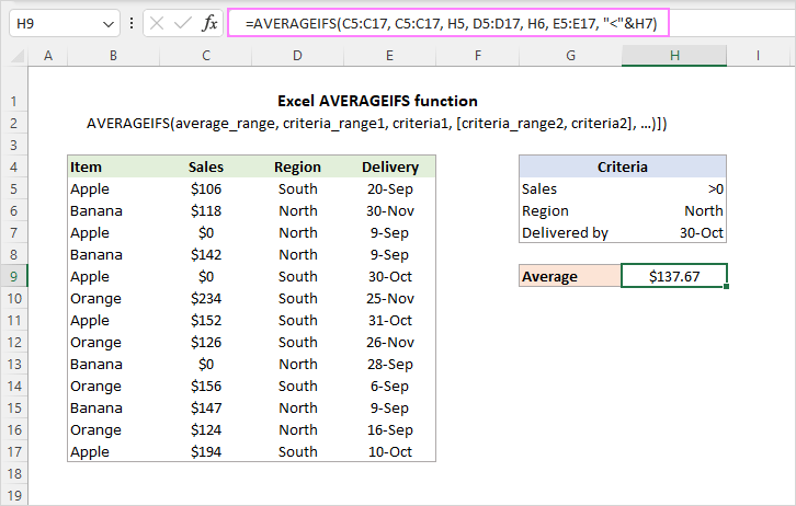
Note. The AVERAGEIFS function works with the AND logic, i.e. only those cells are averaged for which all the conditions are TRUE. To calculate cells for which any single condition is TRUE, use the AVERAGE IF OR formula.
AVERAGEIFS function - usage notes
To get a clear understanding of how the function works and avoid errors, take notice of the following facts:
- In the average_range argument, empty cells, logical values TRUE/FALSE, and text values are ignored. Zero values are included.
- If criteria is an empty cell, it is treated as a zero value.
- If average_range doesn't contain a single numeric value, a #DIV/0! error occurs.
- If no cells meet all of the specified criteria, a #DIV/0! error is returned.
- AVERAGEIFS' criteria may apply to the same range or different ranges.
- Each criteria_range must be of the same size and shape as average_range, otherwise a #VALUE! error occurs.
Now that you know the theory, let's see how to use the AVERAGEIFS function in practice.
Excel AVERAGEIFS formula
First, let us outline the generic approach. To construct an AVERAGEIFS formula correctly, please follow these guidelines:
- In the first argument, supply the range that you want to average.
- In subsequent arguments, specify range/criteria pairs. The pairs can be arranged in any order, but the criteria always follows the range it applies to.
- An AVERAGEIFS formula should always contain an odd number of arguments: average_range + one or more criteria_range/criteria pairs.
AVERAGEIFS with text criteria
To get an average of numbers in one column if another column(s) contains certain text, use that text for criteria.
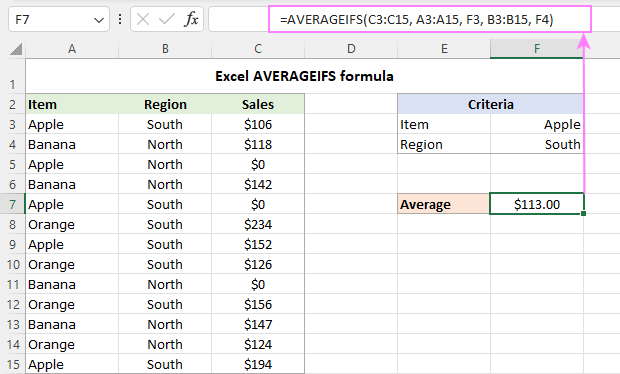
As an example, let's find an average of the "Apple" sales in the "North" region. For this, we make an AVERAGEIFS formula with two criteria:
- Average_range is C3:C15 (cells to average).
- Criteria_range1 is A3:A15 (Items to check) and criteria1 is "apple".
- Criteria_range2 is B3:B15 (Regions to check) and criteria2 is "north".
Putting the arguments together, we get the following formula:
=AVERAGEIFS(C3:C15, A3:A15, "apple", B3:B15, "north")
With criteria in predefined cells (F3 and F4), the formula takes this form:
=AVERAGEIFS(C3:C15, A3:A15, F3, B3:B15, F4)
AVERAGEIFS with logical operators
When the criteria default to "is equal to", the equality sign can be omitted, and you simply put the target text (enclosed in quotation marks) or number (without the quotation marks) in the corresponding argument like shown in the previous example.
When using other logical operators such as "greater than" (>), "less than" (<), not equal to (<>), and others with a number or date, you enclose the whole construction in double quotes.
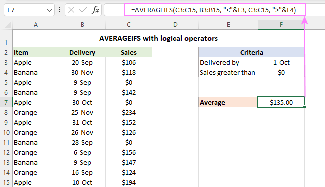
For example, to average sales greater than zero delivered by 1-Oct-2022, the formula is:
=AVERAGEIFS(C3:C15, B3:B15, "<10/1/2022", C3:C15, ">0")
When the criteria are in separate cells, you enclose a logical operator in quotation marks and concatenate it with a cell reference using an ampersand (&). For example:
=AVERAGEIFS(C3:C15, B3:B15, "<"&F3, C3:C15, ">"&F4)
AVERAGEIFS with wildcard characters
To average cells based on partial text match, use wildcard characters in criteria - a question mark (?) to match any single character or an asterisk (*) to match any number of characters.
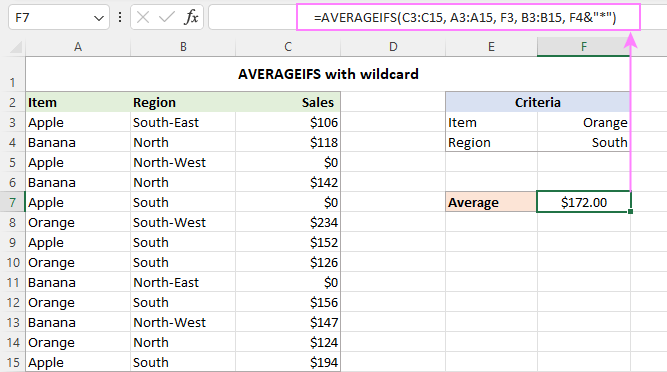
In the table below, suppose you wish to average "orange" sales in all "south" regions including "south-west" and "south-east". To have it done, we include an asterisk in the second criteria:
=AVERAGEIFS(C3:C15, A3:A15, F3, B3:B15, "south*")
If a partial text match criteria is input in a cell, then concatenate a wildcard character with the cell reference. In our case, the formula takes this shape:
=AVERAGEIFS(C3:C15, A3:A15, F3, B3:B15, F4&"*")
Average if between two values
To get the average of values that fall between two specific values, use one of the following generic formulas:
Average if between two values, inclusive:
Average if between two values, exclusive:
In the 1st formula, you use the greater than or equal to (>=) and less than or equal to (<=) logical operators, so the boundary values are included in the average.
In the 2nd formula, the greater than (>) and less than (<) logical criteria exclude the boundary values from the average.
These formulas work nicely or both scenarios - when the cells to average and the cells to check are in the same column or in two different columns.
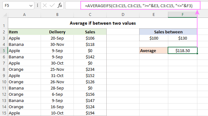
For example, to calculate the average of sales between 100 and 130 inclusive, you can use this formula:
=AVERAGEIFS(C3:C15, C3:C15, ">=100", C3:C15, "<=130")
With the boundary values in cells E3 and F3, the formula takes this form:
=AVERAGEIFS(C3:C15, C3:C15, ">="&E3, C3:C15, "<="&F3)
Please notice that in this case we use the same reference (C3:C15) for the 3 range arguments.
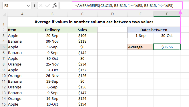
To average cells in a given column if the values in another column fall between two values, supply a different range for the average_range and criteria_range arguments.
For instance, to average the sales in column C if the date in column B is between 1-Sep and 30-Oct, the formula is:
=AVERAGEIFS(C3:C15, B3:B15, ">=9/1/2022", B3:B15, "<=10/30/2022")
With cell references:
=AVERAGEIFS(C3:C15, B3:B15, ">="&E3, B3:B15, "<="&F3)
That's how you use the AVERAGEIFS function in Excel to find an arithmetic mean with multiple criteria. I thank you for reading and hope to see you on our blog next week!
Practice workbook for download
Excel AVERAGEIFS function - examples (.xlsx file)
 by
by
43 comments
I am to create a dynamic average formula. For example, I have 20 employees. I need to calculate a value for each employee based on the average of other employee hours with a specific word in their classification. This is what I have so far, but it is erroring out.
=AVERAGEIFS(C2:C30-C2,A2:A30, A2, B2:B30,"mechanic*")
=AVERAGEIFS(C2:C30-C3,A2:A30, A3, B2:B30,"mechanic*")
=AVERAGEIFS(C2:C30-C4,A2:A30, A4, B2:B30,"mechanic*")
Name Classification Hours
Storm, Sue Lead Mechanic 284
Kent, Clark Chief Mechanic 257
Wayne, Bruce Mechanic 309.25
Parker, Peter Lead Mechanic 452.7
Richards, Reed Mechanic 277.5
Wilson, Wade Lead Mechanic 420.5
Jameson, J Jonah Trainer 342.5
Strange, Stephen Helper 312.75
Stark, Tony Helper 441.5
Hello Dawn!
If I understand the question correctly, you can calculate the average value for all employees who have a specific word in their classification, except for the employee in the current row, using the following formula
=AVERAGEIFS(C2:C30,A2:A30, "<>"&A2, B2:B30,"*mechanic*")
one more question...
I am getting a calculation even when "mechanic" is not found. It is returning a value of 430.23 - I thought if I threw in a "" after the first reference it would only calculate if the value of column C cells were greater than zero, but I can't get it to work.
=AVERAGEIFS(C2:C30,"",A2:A30, ""&A2, B2:B30,"*mechanic*")
OR
=AVERAGEIFS(C2:C30,">0",A2:A30, ""&A2, B2:B30,"*mechanic*")
Hi! These formulas are written incorrectly and cannot work. I could not get the result you are writing about.
If you want results only for rows where you find the word "mechanic" in column B, search for that word with the SEARCH function and use the result "found" in the IF function.
Based on the information given, the formula could be as follows:
=IF(ISNUMBER(SEARCH("mechanic",B2)),AVERAGEIFS($C$2:$C$30,$A$2:$A$30, "<>"&A2, $B$2:$B$30,"*mechanic*"),"")
For more information, please read: How to find substring in Excel
Perfect! Thank you SO much!
Hi!
Is there a way to find the average of a range that is not completely filled in? The range is set, but the data is inputted daily until the end of the year and a running average is needed.
The formula mentioned references a day of the week and averages the data that way
=AVERAGEIF('Data'!R6:R369, Scorecard!D26) where D26 is the day of the week
Currently, only R6:R118 have data, but more is added every day by the user until the end of the year at R369
Thanks!
Hi! To ignore blank and null cells when calculating the average value, add another condition "<>0" to the formula. Read more here: Excel average if not zero or blank.
That worked beautifully! Thank you so much!
Hello again!
I want to add another condition to exclude outliers in the formula while still looking at specific days of the week.
Currently I have:
=AVERAGEIFS('Data'!$J$6:$J$369, 'Data'!$D$6:$D$369, Scorecard!D26, 'Data'!$J$6:$J$369, "")
where
=AVERAGEIFS(data I want to pull, range for the days of the week, day of the week specified, data I want to pull, not null)
I figure the QUARTILE function might work well, but I'm not sure how to nest it into my current formula:
=QUARTILE('Data'!$J$6:$J$369, 3)-QUARTILE('Data'!$J$6:$J$369, 1)
Currently this is for the whole data set, not by weekday
Thanks in advance! Any other function suggestions are also welcomed, it doesn't have to be QUARTILE if something else would work better
=AVERAGEIFS('Data'!$J$6:$J$369, 'Data'!$D$6:$D$369, Scorecard!D26, 'Data'!$J$6:$J$369, "")
Sorry, correcting typo in my original formula
Hi! Unfortunately I'm not quite sure what you want to do. If you want to change the data from which you are averaging with the AVERAGEIFS function to another Excel function, do so in a new, separate column and use a reference to that column in the AVERAGEIFS function.
If you want to count only those data that are greater than the first quartile, add another condition to the formula
">" & QUARTILE('Data'!$J$6:$J$369, 1)
It seems like that works! Can you proofread this formula just to make sure it makes sense?
=AVERAGEIFS('Data'!$J$6:$J$369, 'Data'!$D$6:$D$369, Scorecard!D26, 'Data'!$J$6:$J$369, "", 'Data'!$J$6:$J$369, ">" & QUARTILE('Data'!$J$6:$J$369, 1), 'Data'!$J$6:$J$369, "<" & QUARTILE('Data'!$J$6:$J$369, 3))
Thanks again!
Hi,
I want to use =AVERAGEIF on a non-continuous range. Is that possible?
For example,
=AVERAGEIF((A1,C1,E1,G1,I1,K1,M1),"8888")
Would this formula be possible? Is there any other way to do this?
Correction* the formula I tried but failed was the one below:
=AVERAGEIF((A1,C1,E1,G1,I1,K1,M1),("8888"))
Hi! The AVERAGEIFS function calculates the average value in only one data range, as you can read in the article above.
Hi! I'm trying to incorporate 2 labels from the same column into my AVERAGEIFS:
I have a column that I want to average, and a separate column where I want to only associate certain labels. Here's how I've written it:
=AVERAGEIFS(P2:P36, B2:B44, "="&"Regional", B2:B44, "="&"District")
The items I want to average are (P2:P36), and the labels from B2 I want to average (together) contain the label "District" & "Regional"
Using this method, I received a "value" error. I cannot figure out what the discrepancy is and was wondering if it's because there's blanks in the P column data.
Hi! The discrepancy is that the ranges P2:P36 and B2:B44 are different sizes. They should be identical.
Hello all,
I'm trying to calculate the average over multiple sheets (=average(sheet1:2!AC103:AC60000), but only if the text in column E is "EHP" or "HEH" (the third option is "THP"). Does anyone have a suggestion to do this? Thank you.
Hi! With the AVERAGEIFS function, you can do the average calculation by conditions. However, this function is not included in this list of functions: Excel functions supporting 3-D references. So use the AVERAGEIFS function separately for each worksheet as described in the article above. Then summarize these results.
Can you please give a formula to calculate the average of values in cell B. Until the next row is non blank in cell A.
Hi! Please re-check the article above since it covers your task. Here is an example formula:
=AVERAGEIFS(B1:B5,A1:A5,"<>""")
Hi, I'm wondering there's a way to user AVERAGEIFS with a criteria that looks at part of the data in a cell.
I have this data and want to find the average year (column A) for a range of Dewey classification numbers.
2017 155.90
2018 155.40
2019 155.40
2015 158.11
2010 158.10
2013 158.60
2016 158.20
1998 201 ROS
2016 212 BRO
1992 292.1 QUE
2003 292 EVA
However, some of these classification number also contain letters, which is messing with my criteria. I really only need to compare using the first three digits of the classification number, so for 158.11, 158 is enough to work with. My AVERAGEIFS works beautifully if I create a new column with =VALUE(LEFT(B32,3)) so that I just see these first three digits. This formula =AVERAGEIFS(A2:A1000,D2:D1000,">=100",D2:D1000,"<200") is lovely - but I don't really want to have to create this additional column. Is there a way I can get AVERAGEIF to work directly with my column B data?
Thanks!
Hi! If I understand your task correctly, the following formula should work for you:
=SUM(IFERROR(A2:A1000*(--LEFT(B2:B1000,3)>=100) * (--LEFT(B2:B1000,3)<=200),"")) / SUM(IFERROR((--(LEFT(B2:B1000,3))>=100) * (--LEFT(B2:B1000,3)<=200),0))
Hello,
I am trying to do an averageif function that also has concatenated criteria, but it is across a small range of cells so in an instance or two there will be no values matching that criteria. Is there a way I can nest the function instead of it just returning the #DIV/0 error.
Here is the formula I'm using
=AVERAGEIF(Log!M4:M25,"PS*",Log!AB4:AB25)
to summarize I need the formula to return an n/a when there are no "PS" present in the range of criteria data
Hi! With the IFERROR function, you can show any other value instead of an error message. For example:
=IFERROR(AVERAGEIF(Log!M4:M25,"PS*",Log!AB4:AB25),"N/A")
Read more: How to use IFERROR in Excel with formula examples.
Hi. I have a problem I'm trying to just find the average of 2 numbers in cells AD2 and AG2. I have numbers in between those cells that I don't want to include. I could just use the regular average function and select the two cells I want but I don't want to include any cells that have a value of zero. So I've tried the following code:
=AVERAGEIF(AD2, AG2, "0"). Excel doesn't seem to like that so I've tried =AVERAGEIF(AD2:AG2, "0") but that of course includes all cells between AD2 and AG2 which I don't want. I've tried searching everywhere for a solution but can't find one. Please help if you can. Thanks in advance!
Hi! I don't really understand why you don't want to use the regular AVERAGE function. Zero does not affect the result of the average calculation. I'll take a guess and use IF AND formula:
=IF(AND(AD2>0,AG2>0),AVERAGE(AD2,AG2),"")
Hi thanks for your reply. The average formula does take into account values of 0. If you input 0 into A1 and 20 into A2 and take the average, excel calculates it as 0+20/2 = 10. You can try it yourself. That's the reason for my original question.
I tried what you suggested but instead of excluding the zero and calculating the average as normal, it just sees that there is a zero value and doesn't proceed to calculate anything at all. Thanks for your help. This has got me stumped.
Only in the third question you wrote what result you want to get. If you had read the IF AND instructions I recommended, you would have seen that you can replace the empty value "" with any other value you want. For example, AD2+AG2.
Is it possible for criteria to use a function on criteria range? Say I had date-type data in column A and sales data in column B (and some other columns of data), and I wanted to look at only the first days of the month. Could I have a formula that stats out =AVERAGEIFS(B2:B20,DAY(A2:A20),1, ....... )
Hi! You can only use cell range references as criteria_range.
Hi please help. I am trying to find an average of 2 numbers but when i press enter one of the numbers aren't calculated into the equation. So I have C2 with a value of 1.06 and D2 with an average of *2.25*. I imported a table from a website and some of the numbers have asterisks around them and I can't average them with numbers without an asterisk when I do it just spits out the number without any asterisks. So how would I average C2 and D2. Is there a formula to average these 2 numbers one having asterisks around them. I am very new to using this
Hi! Numbers with asterisks are text. To remove asterisks from text, you can use these instructions: How to delete special / unwanted characters in Excel. Then get the numbers using this manual: How to convert text to number in Excel. Here's one of the formulae:
=--SUBSTITUTE(A1,"*","")
What to do if i need to consider the average sales for both apple and bannana in a single formula. Please help
Hi! I hope you have studied the recommendations in the tutorial above. It contains answers to your question.
Hi! I am trying to have many arguments for the averageif but all in the same column
example: for the data below, I want to get an average of the values in column 3 if column 2 is "red" "pink" or "blue". how would i do this?
col 1 // col 2 // col 3
A / blue // 2.5
B // red // 3
A / pink// 2.5
A // grey// 3
c / red// 2.5
B // pink// 3
Hi! Please re-check the article above since it covers your case. For example,
=AVERAGEIFS(C1:C10,B1:B10,"red")
Since AVERAGEIFS only lets you look for 1 criteria per column, you'll need to set up a helper column. i.e.,
=OR(COUNTIF(B3,"red"),COUNTIF(B3,"pink"),COUNTIF(B3,"blue"))
Then make the criteria range the helper column you set up and have your criteria be "TRUE"
Thank you for your quick reply! In this example, that is indeed a good solution. However, some cities do not have that Youth Movement (1). In that case, I need to refer to another Youth movement, but if that movement is also active in one or more of the other cities, it will duplicate the amount of locations and take it into the calculation. I'm sorry if I'm explaining it a bit unclear.
I see that the formatting of my example is staggered unfortunately. Therefore I try it again.
Note: City = Column A, Youth Movement = Column B, Amount of locations = column C.
City (A) - Youth Movement (B) - Amount of locations (C)
Row 1 New York - Youth Movement 1 - 5
Row 2 New York - Youth Movement 3 - 5
Row 3 New York - Youth Movement 5 - 5
Row 4 Sydney - Youth Movement 1 - 3
Row 5 Sydney - Youth Movement 3 - 3
Row 6 Sydney - Youth Movement 4 - 3
Row 7 Sydney - Youth Movement 6 - 3
Hi,
Thanks for all the tutorials. They are of a great help for me.
However, I've got a problem and I can't figure out how to solve it. I want to calculate the average amount of locations of youth movements of several cities, but the problem is that the number of locations given in the collumn is of all the movements, while in the collumn of the youth movements distinguishes between the type of movements, and not every city has the same sort and amount of movements. The result is that the average that I calculate is not the average of the locations in the cities. Here's an example to illustrate my issue:
(A) Place (B) Youth movement (C) Amount of locations
1. New York YM1 5
2. New York YM3 5
3. New York YM5 5
4. Sydney YM1 3
5. Sydney YM3 3
6. Sydney YM 4 3
7. Sydney YM 6 3
So, while the average should be 4, based on my formula, I get 3.86 as a result, because it gives the average of the sum of all locations. Because it is a pretty big datasets with lots of city combinations, it’s almost impossible to calculate it manually. Does anyone has an idea?
Thanks in advance for your help!
Hi! All the necessary information is in the article above. I don't know what average you want to calculate, but here is an example of the formula:
=AVERAGEIFS(C2:C10,B2:B10,"YM1")