The tutorial shows how to make a dropdown list in Excel with simple steps: from a range of cells, named range, Excel table, another sheet. You will also learn how to make an Excel dropdown menu dynamic, editable and searchable.
Microsoft Excel is good at organizing and analyzing complex data. One of its most useful features is the ability to create dropdown menus, which allow users to select an item from a predefined list. Dropdowns can make data entry faster, more accurate and more consistent. This article will show you a few different ways to create a dropdown menu in Excel.
Excel drop down list
Excel drop down list, aka dropdown box or dropdown menu, is used to enter data in a spreadsheet from a predefined items list. When you select a cell containing the list, a small arrow appears next to the cell, so you click on it to make a selection.
The main purpose of using drop down lists in Excel is to limit the number of choices available for the user. Apart from that, a dropdown prevents spelling mistakes and makes data input faster and more consistent.
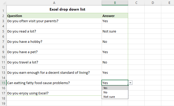
How to create drop down list in Excel
To make a drop-down list in Excel, use the Data Validation feature. Here are the steps:
- Select one or more cells where you want the picklist to appear. This can be a single cell, a range of cells, or a whole column. To select multiple non-contiguous cells, press and hold the Ctrl key.
- On the Data tab, in the Data Tools group, click Data Validation.
- On the Settings tab of the Data Validation dialog box, do the following:
- In the Allow box, select List.
- In the Source box, type the items separated by a comma with or without spaces. Or select a range of cells on the sheet containing the items.
- Make sure the In-cell dropdown box is checked (default), otherwise the drop-down arrow won't appear next to the cell.
- Select or clear the Ignore blank option depending on how you want to handle empty cells.
- When done, click OK.
Congratulations! You have successfully created a simple dropdown list in Excel. Now, your users can click an arrow next to a cell, and then select the entry they want.
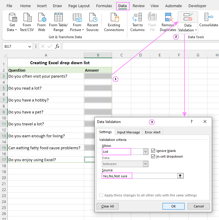
A drop down list of comma separated values works well for small data validation lists that are unlikely to ever change. For frequently updated lists, you'd better use a range or table for the source. The detailed step-by-step instructions for each method follow below.
Tip. To expedite data input in your Excel sheets, you can also use a data entry form.
Make drop-down menu from a range of cells
To insert a drop-down list based on the values input in a range of cells, carry out these steps:
- Start by creating a list of items that you want to include in the drop-down. For this, just type each item in a separate cell. This can be done in the same worksheet as the dropdown list or in a different sheet.
- Select the cell(s) that are to contain the list.
- On the ribbon, click the Data tab > Data Validation.
- In the Data Validation dialog window, select List from the Allow drop-down menu. Place the cursor in the Source box and select the range of cells containing the items, or click the Collapse Dialog icon and then select the range. When done, click OK.
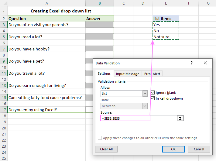
Advantages: You can modify your dropdown list by making changes in the referenced range without having to edit the data validation list itself.
Drawbacks: To add or remove items, you will need to update the Source range reference.
Insert drop down list from a named range
Initially, this method of creating an Excel data validation list takes a bit more time but may save even more time in the long run.
- Make a list of items on the sheet. The values should be entered into a single column or row without any blank cells.
Tip. It's a good idea to sort the items alphabetically or in a custom order you want them to appear in the drop-down menu.
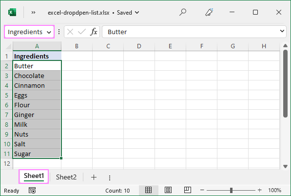
- Create a named range. The fastest way is to select the cells and type the desired name directly in the Name Box. When finished, click Enter to save the newly created named range. For more information, please see how to define a name in Excel.
As an example, let's create a range named Ingredients:
- Select the cells for the picklist - on the same sheet as the named range or in a different worksheet.
- Open the Data Validation dialog window and configure the rule:
- In the Allow box, select List.
- In the Source box, type an equals sign followed by the range name. In our case, it's =Ingredients.
- Click OK.
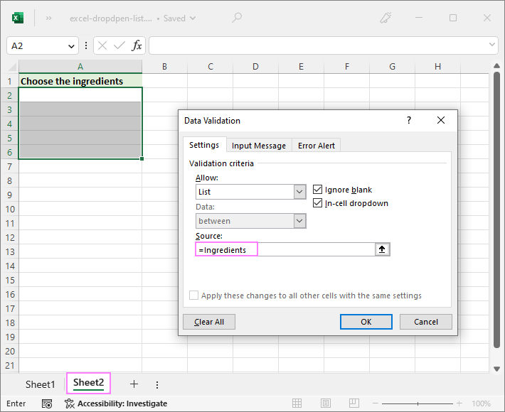
Note. If your named range has at least one blank cell, leaving the Ignore blank box selected allows typing any value in the validated cell.
Advantages: If you insert multiple drop-downs in different sheets, named ranges will make them a lot easier to identify and manage.
Drawbacks: Takes a bit more time to set up.
Create drop-down from Excel table
Instead of using a named range, you can place the source data into a fully functional Excel table. Why may you want to use a table? First and foremost, because it lets you create an expandable dynamic drop-down list that updates automatically as you add or remove items to/from the table.
To make a dynamic dropdown from an Excel table, follow these steps:
- Type the list items in a table or convert an existing range to a table using the Ctrl + T shortcut.
- Select the cell(s) where you wish to insert a dropdown.
- Open the Data Validation dialog window.
- Select List from the Allow drop-down box.
- In the Source box, enter the formula referring to a specific column in your table, not including the header cell. For this, use the INDIRECT function with a structured reference like this:
=INDIRECT("Table_name[Column_name]") - When done, click OK.
For this example, we're making a dropdown menu from the column named Ingredients in Table1:
=INDIRECT("Table1[Ingredients]")
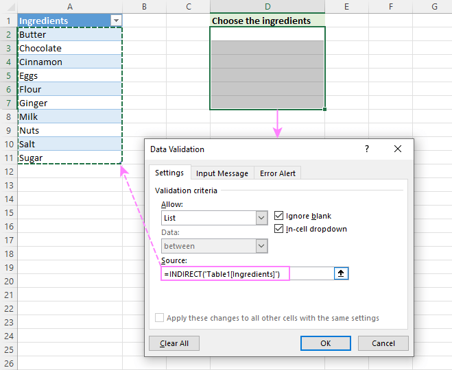
Advantages: Easy and quick way to insert an expandable dynamic drop down menu in Excel.
Drawbacks: Not found :)
How to create a dynamic dropdown list in Excel
If you regularly change the items in your picklist, the best approach is to create a dynamic drop down list. In this case, the list will update automatically in all the cells that contain whenever you add or remove items to/from the source list.
The fastest way to make a dynamic drop down in Excel is from a table as shown above. That is the default behavior of Excel tables; no extra settings or moves are required.
Another way is to use a regular named range and reference it with the OFFSET formula, as explained below.
- Type the items for the drop down menu in separate cells.
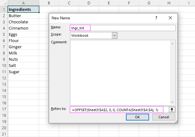
- Create a named formula. For this, press Ctrl + F3 to open the New Name dialog box. Type the name you want in the Name box, and then enter the following formula in the Refers to box.
=OFFSET(Sheet3!$A$2, 0, 0, COUNTA(Sheet3!$A:$A), 1)Where:
- Sheet3 - the sheet's name
- A - the column where the drop-down items are located
- $A$2 - the cell containing the first item
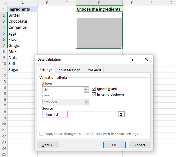
- With the formula name defined, create a dropdown based on a named range as usual.
How this formula works
The formula comprises two functions - OFFSET and COUNTA. The COUNTA function counts all non-blanks in the specified column. OFFSET uses that count for the height argument, so it returns a reference to a range that includes only non-empty cells, starting from the cell containing the first item that you supply for the reference argument.
Advantages: The main advantage of a dynamic drop-down list is that you won't have to change the reference to the named range each time the source list is expanded or contracted. You simply delete or type new entries in the source list, and your dropdown menu will update automatically!
Drawbacks: A bit complex setup process.
Make a dynamic dropdown list in Excel 365/2021
Dynamic Array Excel has many innovative functions that are not available in older versions. One of these new functions named UNIQUE can help you create a dynamic drop-down with a simple formula.
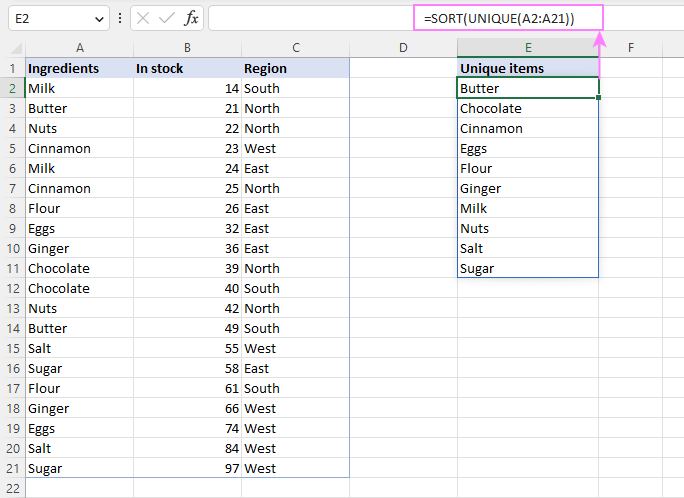
Suppose you have a dataset with many repeated items like in column A in the image below. You aim to add a dropdown list where each item appears just once.
To extract the unique items, use this formula:
=UNIQUE(A2:A21)
Optionally, you can sort the extracted values alphabetically by wrapping it in the SORT function:
=SORT(UNIQUE(A2:A21))
This dynamic array formula is entered just in one cell (E2) and it automatically spills into as many cells as needed to show all the unique items.
Next, you set up a drop down list using a spill range reference, which is a cell address followed by a hash character. In our case it's =$E$2# or =Sheet1!$E$2# if a dropdown is in another sheet:
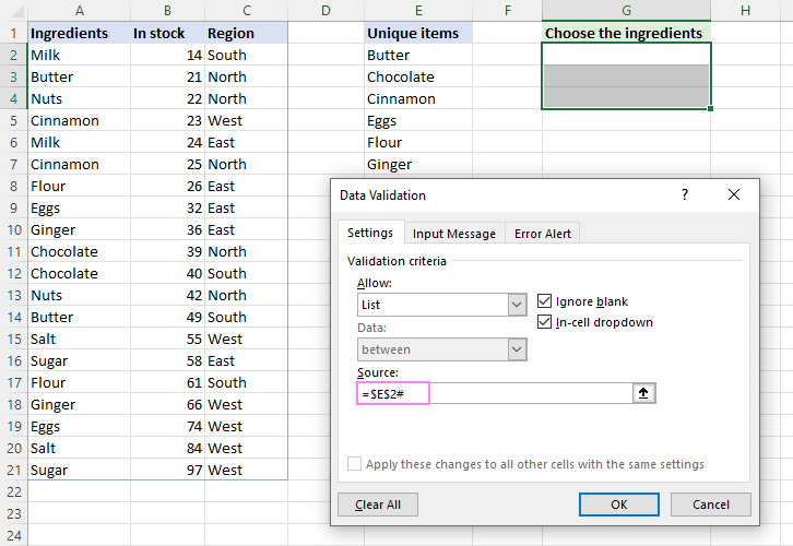
The result is an expandable dynamic drop-down list - the UNIQUE function automatically extracts new items as they are added to the source table, and the spill range reference forces Excel to update the drop-down list accordingly.
Tip. The same approach can be used to create a cascading drop-down list in Excel 365. For full details, please see Make a dynamic dependent dropdown list an easy way.
How to create drop down list from another sheet
To insert a drop-down menu that pulls data from a different worksheet, you can use a normal range, named range or Excel table:
- When making a dropdown menu from a named range, make sure the scope of the name is Workbook, and then set up a data validation list as usual.
- When creating a drop down list from a table, no extra steps are needed as table names/references are valid across the entire workbook.
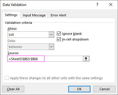
- If you insert a drop down from a regular range, include the sheet's name in the source reference. In the Data Validation dialog window, place the cursor in the Source box, switch to the other sheet and select the range containing the items. Excel will add the sheet name to the reference automatically.
How to make drop-down list from another workbook
To create a drop-down menu in Excel using a list from another workbook as the source, you will have to define 2 named ranges - one in the source workbook and the other in the workbook where you wish to insert your Data Validation list. The steps are:
- In the source workbook, create a named range for the source list, say Source_list.
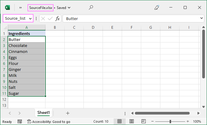
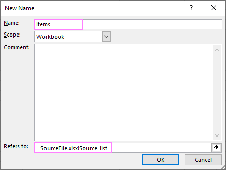
- In the main workbook, define a name that references your source list. For this example, we create the name Items that refers to:
=SourceFile.xlsx!Source_list
If the workbook's name contains spaces or non-alphabetical characters, it must be enclosed in single quotation marks like this:
='Source File.xlsx'!Source_list
For more details, please see How to make external reference in Excel.
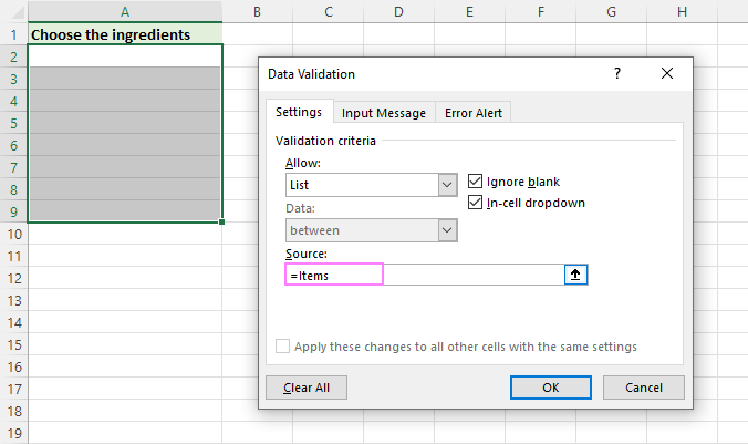
- In the main workbook, select the cell(s) for your picklist and click the Data tab > Data Validation. In the Source box, reference the name you created in step 2. In our case, it's =Items.
Notes:
- For the drop-down list from another workbook to work, the source workbook must be open.
- The dropdown list created in this way won't update automatically when items are added to or removed from the source list - you will have to modify the source list reference manually.
How to make a dynamic dropdown from another workbook
To create a dynamic dropdown list from another workbook, define a formula name in the source workbook using the OFFSET formula explained in Creating a dynamic drop-down in Excel. In this case, a dropdown menu in another workbook will be updated on the fly once any changes are made to the source list.
Searchable drop down list in Excel 365
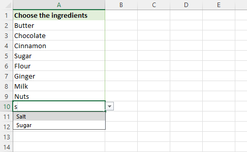
In Excel 365, data validation lists have an awesome AutoComplete feature. To speed up data entry in large lists, just start typing the target word in the dropdown menu cell - the autocomplete algorithm will match the typed substring with the dropdown list items and show you the found matches. As you type more characters, the displayed list is narrowed down, and conversely, when you remove characters, more matches are shown.
Insert a drop down list with message
To show an information message when someone clicks a dropdown list cell, proceed in this way:
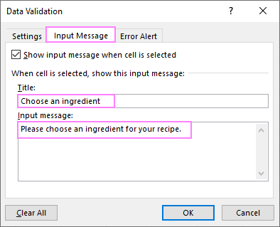
- In the Data Validation dialog box, switch to the Input Message tab.
- Make sure the Show input message when cell is selected option is checked.
- Type the title and message in the corresponding fields (up to 225 characters).
- Click OK to save the message and close the dialog.
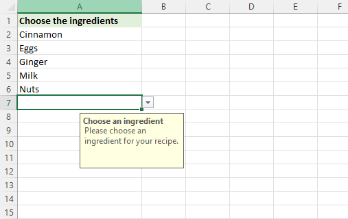
The resulting drop down list with message will look similar to this:
Make an editable drop down list in Excel
By default, an Excel drop-down is non-editable, i.e. restricted to the values in the list itself. If you type any other value, an error alert will show up. However, you can allow users to enter their own values. Here's how:
- Open the Data Validation dialog window.
- On the Error Alert tab, uncheck the Show error alert after invalid data is entered box.
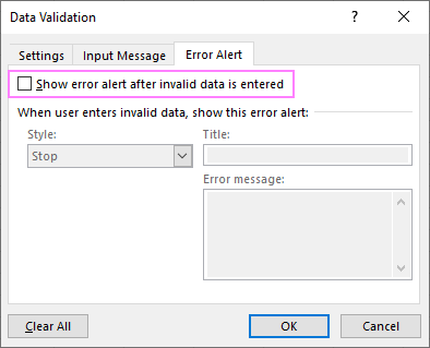
Technically, this turns a drop-down list into a combo box. The term "combo box" means an editable dropdown that allows users to either select a value from the predefined list or type a custom value directly in the box.
Optionally, you can display a warning message when someone attempts to enter a value that is not in the list:
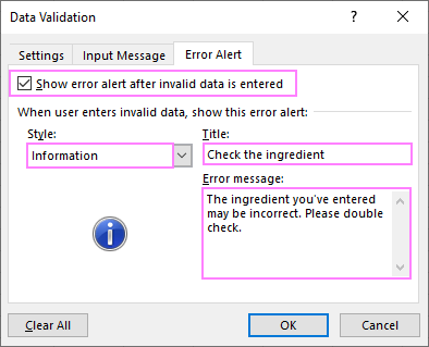
- On the Error Alert tab, select the Show error alert after invalid data is entered option.
- From the Style box, pick either Information or Warning, and then type the title and message text.
- Information message is best to be used if there is nothing wrong with the user entering a custom value.
- Warning message will induce users to select an item from the drop-down box rather than enter their own data, though it does not prohibit it.
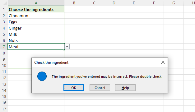
And here's an editable Excel dropdown list with a warning message in action:
Tip. If you are not sure what title or message text to type, you can leave the fields empty. In this case, Excel will display the default alert "This value does not match the data validation restrictions defined for this cell."
That's how to make a simple drop-down list in Excel. In the next article, we will explorer this topic further and learn how to insert a cascading (dependent) drop down list with conditional Data Validation. Please stay tuned and thank you for reading!
Practice workbook for download
Excel drop-down list - examples (.xlsx file)
 by
by
258 comments
This is very helpful.
Hi,
Great article.
I am looking to create a drop down list as described. However using this example I want to be able to pick ingredients from a list of ingredient names in the drop down box (flour, eggs etc). On doing so I want it to represent a price to be used in another formula. So for example if flour cost £1 I want to select the word flour but for it to input £1 in the cell.
Please help.
In search box not a cell
drop doun list in side of box like
thank you
thumps up. GREAT!
Thank you very much for the postings. I have always leant alot from your work. However am wondering whether there is some source of data you can provide on which we can practice on these steps provided.I am still a student and have not have much access to data on which to practice on. I would be more than greatful to be provided with something. Thanks again.
Hello,
I have a large data set for the drop down menu is there anyway to type the name of the specific data I'm looking for instead of trying to scroll down to find it?
Thank you
Hi,
I have the problem that the drop-down list does not work after I sent the excel spreadsheet as a template to my co-workers in order for them to enter their data.
What can be the reason for this behaviour and how do I fix this?
Thanks.
Hi all
is it possible to make drop down list with content which will be depended on the input of another drop down list? for example I have two drop down lists, in the 1st list I have "Cars" and "Phones". If I will choose "Cars" in the 1st list, I want in the 2nd list to appear only "BMW", "Toyota", "Mazda"; if I will select in the 1st list "Phones", I want in the 2nd list to appear only "Samsung", "Nokia", Motorola".
Can anybody help me on this issue?
Thank you in advance.
hello
how can i make a drop down list by default show "--SELECT--" when user open the excel file?
Thanks This has really helped me with my work!
hello
i want to know is it possible for a drop down list to filter data by pressing keys for example i want to see all the word starting from A when i open list and press A and similarly for other alphabets
hello
thank you for your insight. I am attempting to create a drop down menu that is color coded. How do I do this? I not able to find the instructions. My lists are simply words without the coloring.
thanks.
Hi,
I have a query as below:
I'm trying to create a pricing spreadsheet that has headings like "Course group", "Course name", number of users, Price etc. Under the heading "course group", I created a drop down list of all the "course groups" that I have like accounting, asset management etc. Now under the next heading "Course Name", I want to get a specific set of options (course names) in the drop down when I select Accounting for example under the heading "Course Group". How can this be done?
Thanks
thank you somuch for this tutorial, this is very helful for me because I am a documents controller, I really need this, thank you...!
Creating a drop down list is new to me but after reading articles, it appears fairly easy to create. My question is how do I make that drop down list automatically appear in every cell in the column to infinity? I believe that there are not only issues with using control C and control V, but also that only copies the cells selected and my worksheet will grow. In addition, does inserting a row work? Or is it better enter the information on the last row and then sort the data?
I am creating a spreadsheet with multiple columns of drop down lists. The user will sometimes copy and paste their data into the spreadsheet, so I don't want a warning box to come up for every cell of data that doesn't match what is in the drop down. Can I just turn that data red instead of popping up a message? Then, the user can quickly scan for the red data and determine if the data needs to be changed or not. Thank you for your help.
Hi,
i have 2 drop down list in excel. in first drop down list value is 1 to 5 and second list A to E. give me solution that if i select "A" in drop down list than value in first drop down list will show "1" and so on for other.
Thanks.
Hi,
I am using the drop down list for a time sheet style workbook where a user continuously enters time information and selects a job from a drop down list, which is then totalled up on a summary tab.
The problem I have is some jobs change names at some point, so I need to change the name in the list. The name is changed in the drop down list, however all previously entries remain as they were when they were entered (the old job name).
Is there a way to dynamically update the selections of previous entries?
Thanks.
I have three drop down list use the name range
when the first list is category and the others two list depend to show what they contains on the first what, and I realize that I misspelled some category and I correct the name range but the existing cells didn't update
how I can fix that ?
thank you for this information on this website - wondering when creating a list, where do I go to allow the user to be able to check more than one option from the dropdown?
Create a dynamic (automatically updated) Excel dropdown does not work
Hi,
I am trying to create a dynamic drop-down list. There are multiple tabs in the workbook - in the first worksheet, users select or enter in information into a column. In the second sheet, I want a drop-down list containing the entries from that column. As users add more entries into the first sheet, the drop-down list on the second sheet needs to reflect that. I tried to create a dynamic drop-down list as described, and it does show additional entries as they are entered, but it also includes all of the blanks from the column on the first sheet, making it a very long list of blanks. How do I fix this and make the drop-down list only contain the information entered by the user?
Thanks!
Hi,
I was wondering if I could create a list which will contain codes and have their respective descriptions but only show the codes when selected.
Please lemme know if its possible.
Thanks,
John
Hi,
I have created a several combo boxes (form control) in my spreadsheet and in the format control, set the input range by selecting a range of cells from Sheet 2 of my document. I have several combo boxes, connected to several different lists. My problem is that if I select the first option from any of the dropdown lists, they do not save. The only way I have found to get around it is to put a blank field at the top of the dropdown list - but not ideal as I don't want people to be able to select the blank option. I could use data validation, but I prefer the look of combo boxes rather than data validation boxes.
Any ideas ?
Thanks
Cathy
Hello,
I am preparing an excel sheet and want to create a set of tabs let say maximum 10 and for a project reference I need to show only 6 tabs instead of 10 , all these tabs have the same informations.
if we need 4 i have to do something to let my workbook show only 4 tabs, next project i need to show 7 so i have to show only 7.
please could you help on this?
Hello Svetlana, Awesome article and much appreciate the responses that you have provided to various users like me.
My situation seems trivial but not addressed in the responses above
I need to create a picklist from a bunch of data residing in multiple columns in multiple sheets. To explain , I have data in 1st worksheet column A1:A10 , D1:D10..then in worksheet 2 Column A1:A10 , C1:C8. I want the picklist to be created in worsheet 3,column H , merging the data for all the 4 column ranges mentioned above. Is that possible ? Thanks much in advance.
This was great information. I use lists in Data Validation all the time. I'm creating a new Price List that has 3 basic pricelists (Named Range). All customers are based off of 1 of these lists then calculated with specific discounts tailored to each customer. I'd like to use a drop-down menu to choose 1 of the basic lists as a base for that customers calculations. I can make a simple formula using only 1 named range, but I'd like the formula to see the drop-down menu choice and use the correct named range. Is this possible? Any help would be greatly appreciated.
Thank you very much, Its always useful for beginners
Hi Svetlana,
This excel drop down article is awesome & very useful.
I'm using it to create my inventory stock list.
But how to further sorting my dynamic stock list to more details like below:-
1st Option: Brand
2nd Option: Item - Dependent on Brand
3rd Option: Model - Dependent on Brand & Item
4th Option: Serial Number - Dependent on Brand,Item & Model.
I have created a document with the drop down lists. The data is regarding enquiries and members leaving our facility. It is organised by date range, occasionally we have to insert more rows within the data. When I insert a row it is losing my ability to use the drop down lists. Is there a way around this? Many thanks
i learn so much with your article
Yes!!! got the information how to edit and add more names if required.
My xls have 3 drop down colums.Now does that causes the xls to store lesser than 65536 rows.Beacause my xls is able to store 21845 rows which means 65536/3=21845.
On opening the xls having more than 21845 gives error "File is corrupt".
Please help with the issue??
Hai,
I'm seeking a solutions for the below mentioned task. Please help me.
I have two xl file called 1 and 2. In this two xl files 1 and 2 include separate working sheet called R1 and R2. In Sheet R2 so many values in A columns (say A0 to A100 - All the 100 cells having values, that means no cells are blank).
Now I want to link each value from Sheet R2 (A0 to A100) to R1's B column.
The problem is that while linking I want to get the result like this. A0 to B0, A1 to B3, A2 to B4, A3 to B6 etc.
Regards,
Jijesh
Hi Svetlana,
Hope you can help me out with the below issue in excel!
I need to enter the values for a dropdown list in a webpage automatically, once clicking the Command button in excel sheet.
For each and every replacement in the dropdown list, the values related to that need to be exported as a excel file.
for further understanding the webpage will look like (https://drive.google.com/file/d/0BwyKq2OBVvcFT3VGWUZvSXRiRE0/view?usp=sharing) please save the file and open with a browser for the GUI.
I'm new to excel VBA & Macro, so i cannot make the data in excel sheet to place it in the dropdown list in that webpage.
Please let me know for further clarification, also if you've any ideas please let me know.
Thanks in advance !
Regards/ Pravin
Thanks Svetlana.
Saving in the XLSX format done the trick.
Cheers :)
Hi there. I am making spreadsheet for payroll using the method " Creating an Excel drop-down list based on a named range ". I fulfilled all steps yesterday creating a template however going back today it seems to not have saved. I receive a message when saving saying
" one or more cells contain data validation rules which refer to values on other worksheets. These data validation rules will not be saved "
Any help would be appreciated :)
Hi James,
This seems to be a known issue if you are working with .xls workbook in a new Excel. If this is the case, please try the following suggestions:
The warning is incorrect, there is no loss of functionality. You can save the file without losing the Data Validation. You can also avoid this message by one of the following workarounds:
1. Save the file in the XLSX format.
2. Uncheck the "Check compatibility when saving this workbook" option.
For more info about this issue, pleasr see:
https://support.microsoft.com/kb/2757267?wa=wsignin1.0
Hi Svetlana,
My workbook uses macros, which the XLSX format does not support. If I chose macro-enabled format then the dynamic data validation method does not work. Looks like i have to choose between the 2.
Any suggestions?
You have a huge mistake in method one. took over a gad damn hour
you do not put the values as instructed in step 3, you highlight the cells with your input there.....
LOL, true though.
In fact, you can do either way - type directly in the Source box or select the cells with your entries. The latter approach is described in "Drop down list based on a range of cells". Or, are you talking about something different?
Thanks for your tutorial ... super clear!
I've made my list, and insisted on only entries that match those in the list ... but my list is long. Can the Excel list automatically limit the visible list as you begin typing ... so if I type "b" ... the list reduced to only those starting with "b", then if I type "o", now the list would only show those starting with "bo". Can it do this?
Thanks in advance
Hi Dion,
As far as I understand you want to have a drop down list with search suggestions like in Google. If so, you can find the steps and the formulas to create such a drop-down in this article:
http://trumpexcel.com/2013/10/excel-drop-down-list-with-search-suggestions/
Hello! I have two columns in Sheet 1 in a workbook. These are "Partner Name" and "Partner Company". I have a Sheet 2 in that same workbook that also has two columns - "Partner Name" and "Partner Company". I created a dynamic drop-down list so that I can populate the "Partner Name" on Sheet 2 with information from Sheet 1. I would like to populate the "Partner Company" column on Sheet 2 when I populate the "Partner Name" company on Sheet 2. In other words, when I enter "Partner A" in the "Partner Name" column on Sheet 2, I would like to enter the Company Name (as listed on sheet 1 in another column) in the "Company Name" on Sheet 2. I want to populate two columns with one selection on Sheet 2. Is this possible? I was looking at VLOOKUP and think maybe I can use that but am not sure how.
Hi Svetlana,
First off thank you for all your advice and effort, its greatly appreciated. I've read through this section as well as some of the links provided herein but have not quite found / understood what I need for my "issue".
I am trying to create a pay sheet for my staff. We have various staff on different pay grades. We have a separate excel sheet with all our staff names, numbers, paygrade, hourly overtime rate and various other details in rows. e.g. A2=name, B2=number, B3=rate, etc.
I would like to, using a drop down list, select the staff member by name and then in the subsequent columns have the required information (number, rate, overtime rate) inserted automatically in the subsequent columns in the pay sheet. e.g. in C11 we select the staff member by name. Once selected we require C11, C12, C13 and C14 in that sheet to be filled with the corresponding information of that staff member.
The rest of the paysheet is fine, it calculates the remuneration with no problems.
Could you also include the formula for getting the data from a separately saved workbook (we have the staff list stored in the cloud).
Thanks in advance!
I have a similar issue so hope to get your questions answered.
We have two options in the drop-down list, Cash and Finance.
If payment is Cash, subsequent columns to show a price less a $399 discount = Total
If payment is Financed, subsequent columns to show the price as the Total
I am debating honing my VBA skills for this one.. Yikes! We will appreciate the assistance!
Ivan, a lookup() function can be used in this case. so in C12 type "=lookup(C11,[RangeWithName],[RangeWithNumber])" And then C13 would be "=lookup(C11,A2:A999,B2:B999)". I don't know how many people you have, but you get the idea. The function searches in part 2 for what was referenced in part 1 (C11) and prints what is in part 3. These would change dynamically even if you had the names in a table and the table got sorted often or whatnot.
It would be possible to reference a seperately saved workbook if instead of referencing that cell, you had the other excel file open and clicked that file instead. You can not move the file or change the name after that, otherwise it won't work!
You don't need VBA to do this.
Whoops i miss typed... the formula is more like:
IF(Offset(Sheet1!$j$40,0,-1)="n", $H$10:$H$11, $H$10:$H$12))
Dont know how i hit the 3 key sorry...
Hello Marvin,
Sorry, I don't quite understand why you use Offset in this formula. Instead, you could use the column() and row() functions to get the row / column number of the current cell. If you can send a sample workbook at support@ablebits.com, we'll try to suggest a proper formula.
Hi I found this very helpful, however i am working on a roster and used data validation so that you cant select a day shift after workking a nighshift (because the hours overlap etc) DATA Validation formula below:
=IF(Offset(Sheet1!$j$40,0,-1)="n", $H$30:$H$11, $H$10:$H$12))
So... H10="n" (night shift), H11= "p" (afternoon shift) and H12="a" (morning shift)
My question is... can you refference the current cell without putting in the cell letter and number (Sheet1!$J$40). because I would hate to have to write the different refference in the validation for each cell (28 days times 50+ users). And the truth is that i have simplified the formula above because it involves more ifs within the if to account for how many shifts are on for that day already.
So again the question is instead of writing Offset(Sheet1!$J$40... can i write something like Offset(CurrentCel... or something like that. so then i can just copy the formula and use if for the 1400 other cells in the roster.
Thanks in advanced.
This artical is very good. I learn alot. Can you please describe the OFFSET formula? Means in which scenarios it use.
Hello Dipsundar,
This is a very good question!
In Microsoft Excel, the OFFSET function returns a reference to a range consisting of a specified number of rows and columns. You can use it in various scenarios when you need to get a dynamic (i.e. continuously changing) range. You can find more details here:
The OFFSET function in more detail
Thanks again for your great question!
Hi. I want to create a drop down list which shows the text for the user to select, but returns an icon based on what's been selected. Can you help? Thx.
Hello Claire,
You need a special macro for this task. Sorry for not being able to help you with this.
Thank you of trying
Hi,
I am wondering if it is possible to use a drop down list which could be then linked to a column of data. For example, if from the drop down list i choose my first value, a blank column of data that i specify will show which i can then enter data into. If I then select the select value from the drop down list, column of data linked to one disappears and allows me to enter responses for value 2 of my drop down list. If i switch back to value 1 from drop down, the data i entered previously should show up. Is this possible? Or would each response have to entered in a different sheet, then an index match formula be used to call up different column responses based on the drop down value?
Thanks in advance
* If I then select value 2 from the drop down list, ...
Hi Alex,
If you need a cascading drop-down (where values in the second drop-down box depend on the selection in the first one), you'll know how to do it in my next article that will be published tomorrow :)
If you want something different, please send a sample workbook with your data to support@ablebits.com and include the expected result. We'll try to help.
Alex,
Just want to let you know that the "Cascading (dependent) Excel drop down list" tutorial is published:
https://www.ablebits.com/office-addins-blog/dependent-cascading-dropdown-lists-excel/
Hopefully, this is what you were looking for.
Hi Svetlana,
The article is great, very cool indeed but I was looking for something alittle different (if at all possible). I sent an email to support@ablebits.com earlier today.
Thanks!
Alex,
I got it, thank you. I've consulted our Excel gurus and regret to tell you that your task cannot be fulfilled using formulas, at least we do not know any way. This can be done using VBA - you need to track changes in "Design change" and update Column D depending on an old / new value. Sorry for not being able to help you with this.
Hi
i'm looking for a solution. In sheet number 1 i have products name,product part number and description. i'm working in sheet number 2 if i enter part number i want description will be auto generate.
is any formula is there? Please help me.
Hi Madhu,
Well, this is not exactly the topic discussed in this article... Still, you can retrieve the description using a simple VLOOKUP formula.
Suppose you have part numbers and descriptions in sheet 1, in columns B and C, respectively, and row 2 is the first row with data. Then if you enter a part number in cell A2 on sheet 2, and copy the below formula in cell B2, you will get the corresponding description in B2:
=VLOOKUP(A2,Sheet1!$B$2:$C$100,2,FALSE)
Please check out our VLOOKUP tutorial for more information.
Hi
Great website! But I'm really a novice with basic excel knowledge. I'm looking for a way to have a dropdown list with a range of numbers and then have it give me a number for that range.
example:
Price Fee
$0-$499 = $115
$500-$999 = $125
$1000-$2999 = $180
and so on. I would like a column to have a drop down list with the price range and another column with the fee associated with the range.
Gabriel,
The drop-down will follow the previous setup for a "static" drop-down, and you should provide the option(s) in the source as follows:
$0-$499, $500-$999, $1000-$2999
In the cell you want the fee associated with the range, an IF statement should work just fine (a bit rudimentary, but for what you want it to do, it should work well and not have any real issues). Use this:
=IF(C3="$0-$499",115,IF(C3="$500-$999",125,IF(C3="$1000-$2999",180,"")))
Replace C3 with whatever cell your drop-down selection is, then format the column to your liking (most likely as a currency).
The IF statement basically checks which drop-down is selected, then assigns a numerical value based on the selection. Hope this helps
i want to know how can i make my drop down box in excel remain forever when i open next time? please assist me