The tutorial will teach you how to remove blank spaces in Excel to give your worksheets a clear and professional look.
Empty cells are not bad if you are intentionally leaving them in right places for aesthetic reasons. But blank cells in wrong places are certainly undesirable. Luckily, there is a relatively easy way to remove blanks in Excel, and in a moment you will know all the details of this technique.
How to remove blank cells in Excel
Deleting empty cells in Excel is easy. However, this method is not applicable in all situations. To keep yourself on the safe side, please be sure to make a backup copy of your worksheet and read these caveats before you do anything else.
With a backup copy stored in a save location, carry out the following steps to delete empty cells in Excel:
- Select the range where you want to remove blanks. To quickly select all cells with data, click the upper-left cell and press Ctrl + Shift + End. This will extend the selection to the last used cell.
- Press F5 and click Special… . Or go to the Home tab > Formats group, and click Find & Select > Go to Special:
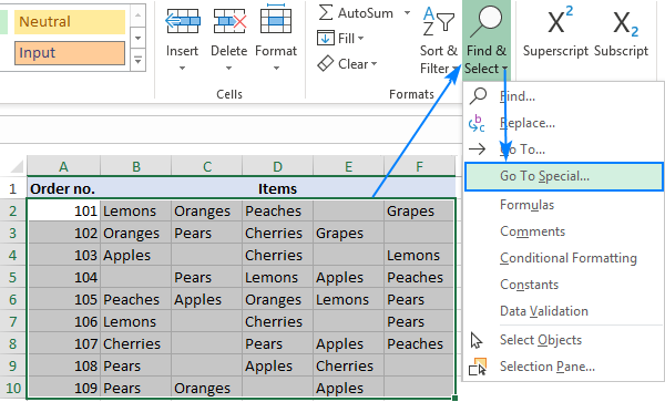
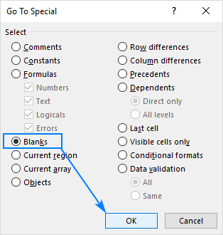
- In the Go To Special dialog box, select Blanks and click OK. This will select all the blank cells in the range.
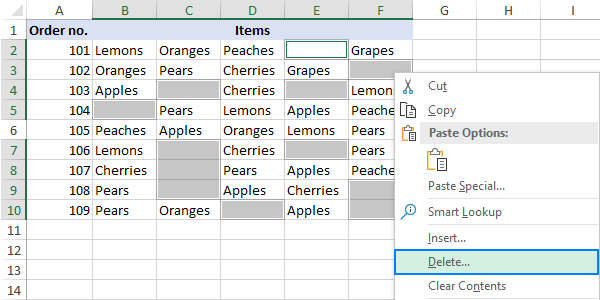
- Right-click any of the selected blanks, and choose Delete… from the context menu:
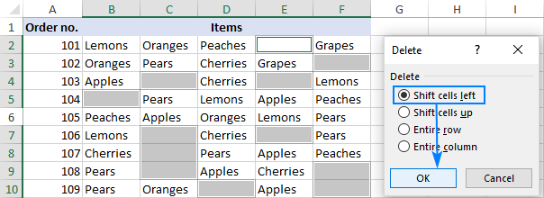
- Depending on the layout of your data, choose to shift cells left or shift cells up, and click OK. In this example, we go with the first option:
That's it. You have successfully removed blank spaces in your table:
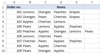
Tips:
- If something has gone awry, don't panic and immediately press Ctrl + Z to get your data back.
- If you only want to highlight blank cells rather than remove, you will find a few different methods in this article: How to select and highlight blank cells in Excel.
When not to remove empty cells by selecting blanks
The Go To Special > Blanks technique works fine for a single column or row. It can also successfully eliminate empty cells in a range of independent rows or columns like in the above example. However, it could be detrimental to structured data. To prevent this from happening, please be very careful when removing blanks in your worksheets and keep in mind the following caveats:
1. Delete blank rows and columns instead of cells
If your data is organized in a table where columns and rows contain related information, deleting empty cells will mess up the data. In this case, you should only remove blank rows and blank columns. The linked tutorials explain how to do this quickly and safely.
2. Does not work for Excel tables
It is not possible to delete any individual cells in an Excel table (vs. a range), you are only allowed to remove entire table rows. Or you can convert table to range first, and then remove blank cells.
3. May damage formulas and named ranges
Excel formulas can adjust to many changes made to the referenced data. Many, but not all. In some situations, the formulas that referred to the deleted cells may get broken. So, after removing blank spaces, take a quick look at the related formulas and/or named ranges to make sure they work normally.
How to extract a list of data ignoring blanks
If you fear that removing blank cells in a column may mangle your data, leave the original column as-is and extract non-empty cells to somewhere else. This method comes in handy, when you are creating a custom list or drop-down data validation list and wish to ensure there are no blanks in it.
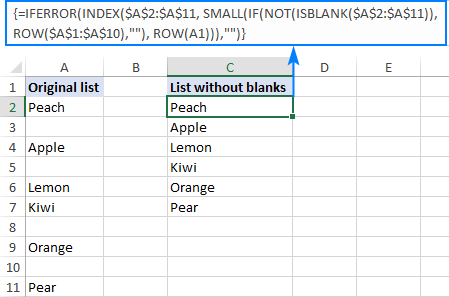
With the source list in A2:A11, enter the below array formula in C2, press Ctrl + Shift + Enter to complete it correctly, and then copy the formula down to a few more cells. The number of cells where you copy the formula should be equal to or greater than the number of items in your list.
Formula to extract non-blank cells:
=IFERROR(INDEX($A$2:$A$11, SMALL(IF(NOT(ISBLANK($A$2:$A$11)), ROW($A$1:$A$10),""), ROW(A1))),"")
The following screenshot shows the result:
How the formula works
Tricky at first sight, upon a closer look the formula's logic is easy to follow. In plain English, the formula in C2 reads as follows: return the first value in the range A2:A11 if that cell is not blank. In case of an error, return an empty string ("").
For thoughtful Excel users, who are curious to know nuts and bolts of every new formula, here's the detailed break-down:
You have the INDEX function return a value from $A$2:$A$11 based on the specified row number (not a real row number, a relative row number in the range). In a simpler scenario, we could put INDEX($A$2:$A$11, 1) in C2, and it would fetch us a value in A2. The problem is that we need to cater for 2 more things:
- Make sure A2 is not blank
- Return the 2nd non-blank value in C3, the 3rd non-blank value in C4, and so on.
Both these tasks are handled by the SMALL(array,k) function:
SMALL(IF(NOT(ISBLANK($A$2:$A$11)), ROW($A$1:$A$10),""), ROW(A1))
In our case, the array argument is generated dynamically in the following way:
NOT(ISBLANK($A$2:$A$11))identifies which cells in the target range are not blank and returns TRUE for them, otherwise FALSE. The resulting array of TRUE and FALSE goes to the logical test of the IF function.- IF evaluates each element of the TRUE/FALSE array and returns a corresponding number for TRUE, an empty string for FALSE:
IF({TRUE;FALSE;TRUE;FALSE;TRUE;TRUE;FALSE;TRUE;FALSE;TRUE}, ROW($A$1:$A$10),"")
ROW($A$1:$A$10) is only needed to return an array of numbers 1 through 10 (because there are 10 cells in our range) from which IF can pick a number for TRUE values.
As the result, we get the array {1;"";3;"";5;6;"";8;"";10} and our complex SMALL function transforms into this simple one:
SMALL({1;"";3;"";5;6;"";8;"";10}, ROW(A1))
As you see, the array argument contains only the numbers of non-empty cells (mind you, these are relative positions of the elements in the array, i.e. A2 is element 1, A3 is element 2, and so on).
In the k argument, we put ROW(A1) which instructs the SMALL function to return the 1's smallest number. Due to the use of relative cell reference the row number goes up in increments of 1 as you copy the formula down. So, in C3, k will change to ROW(A2) and the formula will return the number of the 2nd non-blank cell, and so on.
However, we do not actually need the non-empty cell numbers, we need their values. So, we move forward and nest the SMALL function into the row_num argument of INDEX forcing it to return a value from the corresponding row in the range.
As a finishing touch, we enclose the whole construction in the IFERROR function to replace errors with empty strings. Errors are inevitable because you cannot know how many non-blank cells are in the target range, therefore you copy the formula to a bigger number of cells.
Given the above, we can build this generic formula to extract values ignoring blanks:
Where "range" is the range with your original data. Please pay attention that ROW($A$1:$A$10) and ROW(A1) are constant parts and never change no matter where your data starts and how many cells it includes.
How to delete empty cells after the last cell with data
Blank cells that contain formatting or non-printable characters may cause a lot of issues in Excel. For example, you may end up having a much bigger file size larger than necessary or have a few blank pages printed. To avoid these issues, we will delete (or clear) empty rows and columns that contain formatting, spaces or unknown invisible characters.
How to locate the last used cell on the sheet
To move to the last cell on the sheet that contains either data or formatting, click on any cell and press Ctrl + End.
If the above shortcut has selected the last cell with your data, it means the remaining rows and columns are really blank and no further manipulations are needed. But if it has taken you to a visually empty cell, know that Excel does not consider that cell blank. It could be a mere space character produced by an accidental key stroke, a custom number format set for that cell, or a non-printable character imported from an external database. Whichever the reason, that cell is not empty.
Delete cells after the last cell with data
To clear all content and formatting after the last cell with data, do the following:
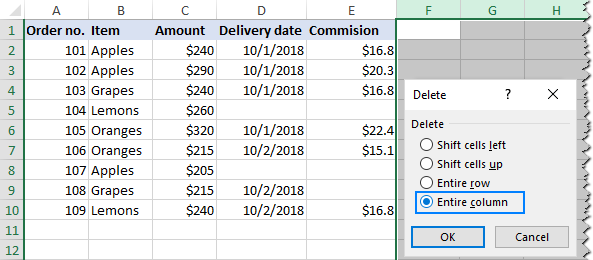
- Click the heading of the first blank column to the right of your data and press Ctrl + Shift + End. This will select a range of cells between your data and the last used cell on the sheet.
- On the Home tab, in the Editing group, click Clear > Clear All. Or right-click the selection and click Delete… > Entire column:
- Click the heading of the first blank row below your data and press Ctrl + Shift + End.
- Click Clear > Clear All on the Home tab or right-click the selection and choose Delete… > Entire row.
- Press Ctrl + S to save the workbook.
Check the used range to make sure it now contains only cells with data and no blanks. If the Ctrl + End shortcut selects a blank cell again, save the workbook and close it. When you open the worksheet again, the last used cell should be the last cell with data.
Tip. Given that Microsoft Excel 2007 and higher contains over 1,000,000 rows and more than 16,000 columns, you may want to reduce the workspace size to prevent your users from unintentionally entering data into wrong cells. For this, you can simply remove empty cells from their view as explained in How to hide unused (blank) rows and columns.
That's how you delete blank in Excel. I thank you for reading and hope to see you on our blog next week!
 by
by
66 comments
I copied this exactly on a brand new spreadsheet and it just returns the list as it is currently, blanks included...
I had the same problem. Even the length of the data in my "blank" cells was zero, but there was clearly something there.
My data was simply text, so I resorted to a simple tactic:
I copied the data into Notepad, and then copied it from there back into my spreadsheet.
Next time I did the operation, the blank cells really were blank, and so the method worked exactly as above.
HTH!
Hi! Here are some other ways to solve this problem: How to delete special / unwanted characters in Excel.
Hi everyone!!
The formula works perfectly as I have tried it. Much thanks to Ablebits Team.
My challenge is;
The formula fails to extract data from a list in a column in which the data have been generated using a formula and not written manually. How can I solve this problem?
Hi Martin this is because the cell has a formula in it and is not blank. I always like to use some kind of error handling mechanism on cells that look empty or have errors and wont have data in them but are not considered empty.
So you will use these tactics on the cell range you evaluating, and not on the formula above.
Using IFERROR(Formula, ""), will cause those cells to be proper blanks although there is a formula in them. If you want zeros also out than you could also do something like this - IF([Certain cell in reference]=0, "", Original formula). That way, even before evaluating the formula, if the primary cell it is reading from is zero, it will be a blank. If reading from multiple cells to derive a value, then do this instead: IF(OR(cell ref1=0,cell ref2=0, cell ref3=0,...), "", Original formula)).
Hope this helps
Hi! To avoid extracting zeros and empty values, change the condition in the formula:
=IFERROR(INDEX($A$2:$A$11, SMALL(IF($A$2:$A$11<>0, ROW($A$1:$A$10),""), ROW(A1))),"")
Hey All,
I have tried to expand the formula to account for both number values and blanks, I did this by expanding the if statement to an "and" and having two checks check if not blank and if not a number, not sure where I have gone wrong here any advice would be appreciated.
=IFERROR(INDEX($A$2:$A$30, SMALL(IF(AND(NOT(ISNUMBER($A$2:$A$30)),NOT(ISBLANK($A$2:$A$30))), ROW($A$1:$A$29),""), ROW(A1))),"")
Hi! If you want to exclude numbers and empty cells, try the ISTEXT function instead of NOT ISNUMBER and NOT ISBLANK.
Great help
Dear Experts,
11088804 18087868 19031819 19670487 22418920 31080665 34417320 36689345
39040804 71259793 72339654 72584638 90229749 95036618
11352073 14731289 18760612 22746837 25008809 28672035 29361465 36405675
55666397 63880914 72273261 72832139
13353870 70503278 72419264 72946319 99392733
11690688 11756662 21042271 25342925 38001290 80393697 85773314 85835326
89027294 89931878 95025519 95058273
73047072
11668225 11698423 12360439 12710342 16034669 21094686 21382219 23341957
26696292 27002716 27012497 27797269 28674338 31080665 33693127 34003028
36999405 45999293 60547937 60548754 62549297 65547590 65877919 66880473
68497914 69879568 70202347 70431025 70655132 70656112 70765323 71181908
71239845 71425671 71654636 71880015 73175190 85786104 85848037 95169607
95178486 99313970 99479700 99556797 99737744 99935068 99997288
this is the data i have it in multiple columns along with empty cells. Please guide me, how to delete blank cells in each column and bring all data in one column. thanks
Hello!
If I understand the problem correctly, to convert a range into one column of data, try the TOCOL function.
Use the formula
=TOCOL(A1:C7,3,TRUE)
You can find the examples and detailed instructions here: Excel TOCOL function - convert range to single column.
The blank cells in my list was filled with (" ") by certain formula that I am using, upon using the the above formula it came out with the same list with blanks (not change), however it worked like a charm by replacing (" ") in the blank cells with number (0) by modifying my original formula.
There is a you tube video that describes how to implement this formula, after pressing (Shift. Alt, Enter) you have to drag down the formula cell to get all the filtered cells in the new list.
Hello!
To avoid showing zero in empty cells, change the format of these cells. Use this guide: Display zeroes as dashes or blanks.
Hi,
I'm using the following formula to extract data from a schedule to return all occupied cells into a list format.
=IFERROR(INDEX($G$5:$G$21, SMALL(IF(NOT(ISBLANK($G$5:$G$21)), ROW($G$1:$G$21),""), ROW(C1))),"")
It's working great for the first column, but I'm trying to figure out how to run the formula for multiple columns where the returned list is still in one column. Does that make sense? I've tried expanding the range within the index but that just returns the data in the other columns under their own separate column. As is in the formula below:
=IFERROR(INDEX($G$5:$H$21, SMALL(IF(NOT(ISBLANK($G$5:$H$21)), ROW($G$1:$H$21),""), ROW(C1))),"")
For example, I have entries in G7, G13, G15, H5, and H10. I want all entries to be recorded in a new list but I only seem to be able to retrieve entries from Column G
Any tips for me?
Hello!
Unfortunately, I was unable to extract non-blank data cells from the range using your formula. If you want to extract data from two columns, excluding blank cells, try this formula:
=FILTER(TOCOL(G5:H13),TOCOL(G5:H13)>0)
Use TOCOL function to convert range to single column. FILTER function extracts all numbers that are greater than zero. You can use any other condition.
I hope it’ll be helpful. If something is still unclear, please feel free to ask.
Greetings. I've been working endlessly trying to get a formula to work. Any assistance would be greatly appreciated.
The formula I'm using is:
=IFERROR(INDEX($D$101:$D$1100, SMALL(IF($D$101:$D$1100 "", ROW($D$101:$D$1100),""), ROW(D100))),"")
and of course I'm clicking ctrl-shft-enter to get the brackets for the formula. {formula}
I've tried copying it down the page a bit and that has zero effect it seems.
My range of data I'm referencing is D101:D1100 with a header in D100.
The formulas in that range are referencing data from another sheet.
Example:
=IF('Test Completion Report'!$J3="Chlorine (Cl)",'Test Completion Report'!$L3,"")
then
=IF('Test Completion Report'!$J4="Chlorine (Cl)",'Test Completion Report'!$L4,"")
etc.
Using those formulas I create the D column range with lots of blank cells containing "", not truly empty, and occasional numbers here and there when matches exist.
I'm trying to get rid of the "blanks" in that D column data and exhibit the resulting table of values in the H column. So I'm putting my formula in H101.
I have multiple columns like that D column for different search terms. Once I get this one formula working I plan to have other formulas to do the same for the other columns.
I think I'm getting close when looking at the Formula evaluation. It gets to the point in the Evaluation of saying
=IFERROR(Index($D$101:$D1100,#Num!),"")
The previous eval step (5th evaluate click if I recall correctly) created the #NUM that is causing failure.
On the steps leading up to the failure it's performing the other steps for false false false true false false etc., then converting those later to the steps saying:
=IFERROR(INDEX($D101:$D$1100, SMALL({"";"":""; etc. then ;108;"";etc. with "" and numbers through to the end, then ending with ;""},100)),"").
The next eval click gets the #Num value as indicated.
I am trying to be absolutely descriptive of what I'm working with, my apologies if I've not been clear enough or alternately rambled more than needed.
I have a sneaking suspicion that it may lie with something like the fact that my first value (in D101) isn't a number, aka not a "true"???
Thank you for your time in the matter.
Dang it, an error in the formula itself when typing it across...... there should be does not equal using less than greater than in there.... I'll try copy paste again...
=IFERROR(INDEX($D$101:$D$1100, SMALL(IF($D$101:$D$1100 "", ROW($D$101:$D$1100),""), ROW(D100))),"")
It shows on the post a comment screen.. so unless it's getting taken out upon send....
...SMALL(IF($D$101:$D$1100 then less than greater than then "", etc.
Yeah, when posting it's stripping the does not equal from the equation....
Hello!
Unfortunately, I was unable to reproduce your problem, and without seeing your data it is difficult to give you any advice. Please provide me with an example of the source data and the expected result.
Does NOT work
Hi!
The recommendations in this article are tested and supported by examples. If you describe your problem, I will try to help you.
Mates, can I ask, is Ablebit suite has a tool for removing blank cells in the range for the Google Sheets (not an offline PC Excel) similar to what was described above in the article here for Excel?
Much appreciated! i'm on a trial currently..btw
Hello George,
As for special tools, at the moment we have only Remove Blank Rows and Columns.
As for the standard Google Sheets solutions, you can either filter cells so only blanks remain or use the QUERY function to get the data without the blanks.
Hi, the formula works fine for the first row: C2 returns "Peach" , but when I copy the formula in C3, C4... C11, the result is only blanks.
ROW (A2) changes with the row, to A3, A4 .. A11; but the result is always blank after C2...
Can you help?
Hello!
Without seeing your formula, I cannot give advice on how to change it. However, I think your problem is relative and absolute cells references. See which references change when copied and check out this guide.
cool trick
I'm wondering is there a formula tweak here. So that on a separate sheet or a separate area if my table or section has blank rows they will not be copied to this other sheet or other section. I am looking for some formula that would copy over a row of information and only those row that are NOT blank. Blank rows would not be copied. In the new section there would be no blank rows. I'm thinking as an example an inventory list. In column A would have the quantity. In column B would have part number. In column C would have description. In column D would have price. That's my master sheet. Call the or my build sheet. I want it to look at the quality column if there is no number there then consider it blank and do not copy it over to the build list but if it is or does have a number then it is not blank and copy it over to the build list. Hope this makes sense thank you very much for your consideration.
Hello!
If I understand your task correctly, you can set a filter on this column and get only rows with values. You can copy these values.
I hope I answered your question. If something is still unclear, please feel free to ask.
with the number of people having issues with this formula working correctly, you'd think you would look to understand why rather than telling people to "go read the post better"
Hello!
If you describe your problem in detail and accurately, we will definitely try to solve it. In your message, as in some others, there is no such information.
hi svetlana ; i want to cut out all blanks entire columns and a i want to equal 1 coulmn to another for example first column 14 67 87 34 second column is i you we they and (this is not a formula i create it in my brain) equal code ( = ) and i use it a first column A second column is B and i use it A=B .
and computer learn it and went to ram and another column is
C= i i i i i we we we we they they they and i use it this formula(this is a not a formula i create it in my brain but excel contain like a these but i dont know please you teach me ) and computer write 14 14 14 14 14 87 87 87 87 34 34 34 and computer wrtie them
please teach these formula to me
sorry for my english my english is bad
Hello.
First, thank you for the great guide. I'm using the formula for extracting a data list while ignoring blanks.
My formula:
=IFERROR(INDEX(BlanksRange,
SMALL(IF(NOT(ISBLANK(BlanksRange)),
ROWS($A$1:$A$10),""),ROW(A1))),"")
When I press Ctrl+Shift+Enter I get only blank cells. I removed the IFERROR to debug.
My debugging formula:
=INDEX(range, SMALL(IF(NOT(ISBLANK(range)), ROW($A$1:$A$10),""), ROW(A1)))
After pressing Ctrl+Shift+Enter I get #N/A on all cells. I'm using a dynamic named range, but I got the same results with the hard referenced $B$2:$B$19 range.
乁( •_• )ㄏ
Any ideas?
The different name for the range on the debugging formula was a mistake here. It should say BlanksRange same as above.
Hello Aristides!
There is a mistake in your formula. Instead of ROWS($A$1:$A$10), write ROW($A$1:$A$10).
Your BlanksRange array should have 10 rows. If not, change the range of $A$1:$A$10.
If the number of rows in your range changes, try this formula
=IFERROR(INDEX(BlanksRange, SMALL(IF(NOT(ISBLANK(BlanksRange)), ROW(INDIRECT("1:" & ROWS(BlanksRange))), ""), ROW(A1))),"")
Hope this is what you need.
Thank you for your response.
I just rechecked the ROWS error was an error by me when typing on my cell phone. My range does change as I keep adding stuff to the main list. I was able to do it with this:
{=IFERROR(INDEX(dynamicRange,
SMALL(IF(LEN(dynamicRange),
ROW(INDIRECT("1:"&ROWS(dynamicRange)))),
ROW(A1)),1,"")}
I was just trying to avoid using volatile functions, but I guess I have no choice on this one.
Again, thanks a lot. ?
The formula works great for the first cell but when I drag down the formula to the other cells I get a blank (if I have IFERROR) or a #NUM! if not. I'm not sure when I am doing wrong. Here is my formula.
=IFERROR(INDEX($G$13:$G$30,SMALL(IF(NOT(ISBLANK($G$13:$G$30)),ROW($A$1:$A$18),""),ROW(A1))), "")
All information is in G13:G30 and I am putting my formula in K13 for right now.
Thanks!
Thank you for sharing. I did the opposite lately. I have to ensure my cells are blanks while submit it for updates to database as it does not take null values.
Hello,
Can you help me pls, i don't know why the formula works only for the first 6 rows and then won't bring any data from the collom I to J
The formula that i am useing:
=IFERROR(INDEX($I$2:$I$3001, SMALL(IF(NOT(ISBLANK($I$2:$I$3001)), ROW($I$1:$I$3000),""), ROW(I1))),"").
Can you help me pls.
Thank you.
Hi! In my workbook, this formula works for all rows. Unfortunately, I don't have your data.
Mine doesn't seem to be working. It grabs the first cell item in the list, but when I drag the formula to the remaining cells below. They just come back blank.
So in Cell C2: =IFERROR(INDEX(A2:A11, SMALL(IF(NOT(ISBLANK(range)), ROW($A$1:$A$10),""), ROW(A1))),"") And it does bring up "Peach"
In Cell C3: =IFERROR(INDEX(A3:A12, SMALL(IF(NOT(ISBLANK(range)), ROW($A$1:$A$10),""), ROW(A2))),"") - Just comes up blank
Cells C4 - C10 are all also blank. The only change in each cell is the last part ROW(A1 to A2... etc)
Hello Thomas!
If I understand your task correctly, the following formula should work for you:
=IFERROR(INDEX($A$2:$A$11, SMALL(IF(NOT(ISBLANK(range)), ROW($A$1:$A$10),””), ROW(A1))),””) And it does bring up “Peach”
You can read more about absolute and relative cell references here.
I hope this will help, otherwise please do not hesitate to contact me anytime.
When I do this, for some reason ROW(A1) always stays as ROW(A1) in every cell throughout the range, whereas it should be A2, A3, A4, etc. in each cell lower down in the array output range. Not sure what I'm doing wrong.
Hello Joe!
If I understand your problem right, you are trying to copy =ROW(A1) down to the other cells in column A. Unfortunately, I can’t reproduce the issue, the formula is copied correctly. It does not change only if it looks like =ROW($A$1). Maybe, you are copying a formula, not a cell. Please describe in more detail what steps you take and we’ll try to find the cause of the issue.
Hello!
I wants to remove formula error(#N/A! or #Num!) cell or formula blank cell, although it's not blank but is it possible? if possible how to do please explain. Thank you.
Hello Al-Amin!
In order not to show errors in cells, the IFERROR function is used. To learn more about it, please read this article on our blog: https://www.ablebits.com/office-addins-blog/excel-iferror-function-formula-examples/
You can use our Ultimate Suite for Excel to search for empty cells with formulas. You can select all cells with formulas in a sheet by using Select by Value -> Select Special Cells. Then you can substitute all selected formulas with their values by using Convert Formulas to Values. All invisible and non-printing characters can be deleted with the help of Remove Characters.
You can install Ultimate Suite in a trial mode and test the tools for 30 days for free: https://www.ablebits.com/files/get.php?addin=xl-suite&f=free-trial
I hope this information will be helpful to you.
Hey,
I want to remove blank cell in excel.
can you guide me how to do it?
Hello!
Please check out the first paragraph of this article: https://www.ablebits.com/office-addins-blog/remove-blank-cells-excel/#delete-blank-cells-in-Excel
For me to be able to help you better, please describe your task in more detail. It’ll help me understand it better and find a solution for you. Thank you.
I can't get this to work for me, unfortunately. Would I be able to send a screenshot of what I'm doing? Everything looks accurate in the formula but its returning a blank cell.
Thanks
your presentation with screen shot is very easy to understand. im happy to learned something. Great and Good Job. Thanks
Hi, What formula could be used to sort items without blank cells, if the range is not vertical (A1:A10), but it is horizontal (A1:K1), for example?
Hi there, I am attempting to use this function to remove blank cells but this only seems to work on the cells after the last cell containing data.
i.e. all blank cells in between data are still there.
Can you please advise?
Hello Warren,
Please see the first 3 sections of this tutorial. They explain how to remove blanks in between data.
Hi,
Your formula is works when the cell is really empty.
But I make a cell empty (visually ONLY) by formula "=IF(A$2=ISBLANK(0);"";A$2".
It means the cell is not really Empty :-)
But I still need the result like in your example "How to extract a list of data ignoring blanks."
Could you please help me this issuer?
I found that using the following tweaked formula helped me accomplish the results better if trying to remove the blank rows that contain formulas where the blank row actually equals "", which is not truly blank.
{=IFERROR(INDEX(range, SMALL(IF(range"", ROW($A$1:$A$10),""), ROW(A1))),"")}
VERY Helpful!!!
I got around Excel not counting a formula as blank because my actual interest is in whether there is a number in the checked cell -- else omit row. Exchanging the "ISBLANK" for "ISNUMBER" fits my need. As well, I created a variable end for the A1:... with an INDIRECT(ADDRESS( ...)) that uses a cell that knows how many rows there are as this changes with each use. Again, works great. Thanks!!!
John
Extremely helpful tutorial and explanations on How to extract a list of data ignoring blanks. However its not working for me. Not yet. The problem is that my data is dynamically changing almost every day and I have it organised as a table. In a certain column there are new data generated daily and also there are blanks every now and then. So how do I adapt the original formula in order to dynamically (automatically) extract a list of data ignoring blanks in daily changing (adding) data? I believe the solution to this problem would be very appreciated from a broader community. Thank you again for this tutorial and kindest regards!
Marjan
Hi, Thank you for the exceptional guide and I find it working for simpler tasks. However, I´m working on a larger project right now.
The goal is to Extract data from a table, only if a certain name is printed. Example if Martin is printed, the idea is for the list to blank/NA() all the info that is not related to Martin.
Example:
Name:
Peter Corn
Martin Pizza
Anna Orange
Isak Pizza
Fredrik Corn
Martin Orange
Peter Corn
Name: Martin Result:
Pizza
Martin Pizza Orange
Martin Orange
The way I handle the problem is that as I use formulas to created the table I can´t use blanks, hence I replace it with NA() and isNA in the formula. There are 106 entries and only 5 of them are needed for the list. Hence it is 101 #N/A and 5 results with names.
I Try to apply the formula as this (In swedish excel ;=,):
{=IFERROR(INDEX($B$3:$B$98; SMALL(IF(NOT(ISNA($B$3:$B$98));ROW($A$1:$A$10);""); ROW(A1)));"")}
Unfortunately, no result is shown. The only way I can get a result is if I put in a value at the top of the list, but that is only without the array function. Any ideas on how I can get it to work on this scale with formulas in the cells?
Regards
Martin
The Example did not, unfortunately, translate well after I pressed send, but the point is only to get out the food chosen by Martin.
Martin, this might be a bit old but in reading, you show row($a$1:$A$10) - this is only referring to the top 10 positions in the list not 95 like you need, should change to row($a$1:$A$95)
95 = 98-3 .
Hello raggazzi! (Italian for ""guys and gals" :-)>
First, I want to say that the ablebits.com website is outstanding; not only in terms of Excel expertise, but also in the clarity of presentation and "style" of written english. Bravo!
I have one problem, however, with
"How to extract a list of data ignoring blanks"
from https://www.ablebits.com/office-addins-blog/remove-blank-cells-excel/
This is an elegant formula, but for me it only seems to work when I start it exactly as shown, at cell A1. If I attempt to move it, or even simply insert a row above, so that it begins on Row 2 at A2, it doesn't work. I've tried working with relative vs absolute addresses, etc. but no luck. Am I missing something?
Thanks again,
Howard
Hi Howard,
Thank you for your kind words about our blog, it's a good incentive for us to keep it up :)
Regarding the formula. In fact, in our example, the data starts in cell A2 (A1 is the column header and it's ignored by the formula). The logic is explained in the "How the formula works" section that comes right after the example. To adjust the formula for your data, be sure to change only "range" in the generic formula below, and remember to press Ctrl+Shift+Enter to complete it:
IFERROR(INDEX(range, SMALL(IF(NOT(ISBLANK(range)), ROW($A$1:$A$10),""), ROW(A1))),"")
For example, if your data starts in rows 3, i.e. range=$A$3:$A$12 (mind the absolute references!), the formula would go as follows:
=IFERROR(INDEX($A$3:$A$12, SMALL(IF(NOT(ISBLANK($A$3:$A$12)), ROW($A$1:$A$10),""), ROW(A1))),"")
This does not appear to work with results from formulas. I have used an if condition to blank out many rows that are not needed. Trying to remove those rows using this does not seem to work.
Hi Dustin,
You are right, this does not work with formula results. In terms of Excel, a cell containing a formula is not blank even if the formula returns an empty string.
A solution would be to code blanks in your formula results as 'NA()', then replace 'ISBLANK()' with 'ISNA()' in the formula above.
Hi there thanks for the guide, how would you apply this to multiple columns? If this is not possible, is there a simple way to combine columns where this approach has been used multiple times. Many thanks.
Ed