The tutorial explains the Excel REPLACE and SUBSTITUTE functions with examples of uses. See how to use the REPLACE function with text strings, numbers and dates, and how to nest several REPLACE or SUBSTITUTE functions within one formula.
Last week we discussed various ways of using FIND and SEARCH functions within your Excel worksheets. Today, we will be taking a deeper look at two other functions to replace text in a cell based on its location or substitute one text string with another based on content. As you may have guessed, I am talking about the Excel REPLACE and SUBSTITUTE functions.
Excel REPLACE function
The REPLACE function in Excel allows you to swap one or several characters in a text string with another character or a set of characters.
As you see, the Excel REPLACE function has 4 arguments, all of which are required.
- Old_text - the original text (or a reference to a cell with the original text) in which you want to replace some characters.
- Start_num - the position of the first character within old_text that you want to replace.
- Num_chars - the number of characters you want to replace.
- New_text - the replacement text.
For example, to change the word "sun" to "son", you can use the following formula:
=REPLACE("sun", 2, 1, "o")
And if you put the original word in some cell, say A2, you can supply the corresponding cell reference in the old_text argument:
=REPLACE(A2, 2, 1, "o")

Note. If the start_num or num_chars argument is negative or non-numeric, an Excel Replace formula returns the #VALUE! error.
Using Excel REPLACE function with numeric values
The REPLACE function in Excel is designed to work with text strings. Of course, you can use it to replace numeric characters that are part of a text string, for example:
=REPLACE(A2, 7, 4, "2016")

Notice that we enclose "2016" in double quotes as you usually do with text values.
In a similar manner, you can replace one or more digits within a number. For example:
=REPLACE(A4, 4, 4,"6")
And again, you have to enclose the replacement value in double quotes ("6").
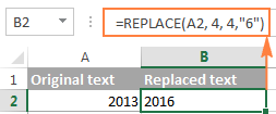
Note. An Excel REPLACE formula always returns a text string, not number. In the screenshot above, notice the left alignment of the returned text value in B2, and compare it to the right-aligned original number in A2. And because it's a text value you won't be able to use it in other calculations unless you convert it back to number, for example by multiplying by 1 or by using any other method described in How to convert text to number.
Using Excel REPLACE function with dates
As you have just seen, the REPLACE function works fine with numbers, except that it returns a text string :) Remembering that in the internal Excel system, dates are stored as numbers, you may try to use some Replace formulas on dates. Results would be quite embarrassing.
For instance, you have a date in A2, say 1-Oct-14, and you want to change "Oct" to "Nov". So, you write the formula REPLACE(A2, 4, 3, "Nov") that tells Excel to replace 3 chars in cells A2 beginning with the 4th char… and got the following result:
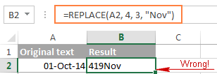
Why's that? Because "01-Oct-14" is only a visual representation of the underlying serial number (41913) that represents the date. So, our Replace formula changes the last 3 digits in the above serial number to "Nov" and returns the text string "419Nov".
To get the Excel REPLACE function to correctly work with dates, you can convert dates to text strings first by using the TEXT function or any other technique demonstrated in How to convert date to text in Excel. Alternatively, you can embed the TEXT function directly in the old_text argument of the REPLACE function:
=REPLACE(TEXT(A2, "dd-mmm-yy"), 4, 3, "Nov")
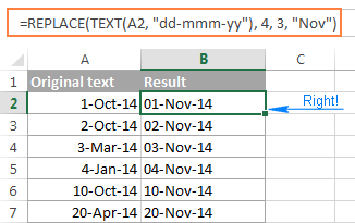
Please remember that the result of the above formula is a text string, and therefore this solution works only if you are not planning to use the modified dates in further calculations. If you do need dates rather than text strings, use the DATEVALUE function to turn the values returned by the Excel REPLACE function back to dates:
=DATEVALUE(REPLACE(TEXT(A2, "dd-mmm-yy"), 4, 3, "Nov"))
Nested REPLACE functions to do multiple replacements in a cell
Quite often, you may need to do more than one replacement in the same cell. Of course, you could do one replacement, output an intermediate result into an additional column, and then use the REPLACE function again. However, a better and more professional way is to use nested REPLACE functions that let you perform several replacements with a single formula. In this context, "nesting" means placing one function within another.
Consider the following example. Supposing you have a list of telephone numbers in column A formatted as "123456789" and you want to make them look more like phone numbers by adding hyphens. In other words, your goal is to turn "123456789" into "123-456-789".
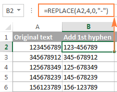
Inserting the first hyphen is easy. You write a usual Excel Replace formula that replaces zero characters with a hyphen, i.e. adds a hyphen in the 4th position in a cell:
=REPLACE(A2,4,0,"-")
The result of the above Replace formula is as follows:
Okay, and now we need to insert one more hyphen in the 8th position. To do this, you place the above formula within another Excel REPLACE function. More precisely, you embed it in the old_text argument of the other function, so that the second REPLACE function will handle the value returned by the first REPLACE, and not the value in cell A2:
=REPLACE(REPLACE(A2,4,0,"-"),8,0,"-")
As the result, you get the phone numbers in the desired formatting:
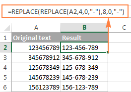
In a similar manner, you can use nested REPLACE functions to make text strings look like dates by adding a forward slash (/) where appropriate:
=(REPLACE(REPLACE(A2,3,0,"/"),6,0,"/"))
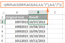
Moreover, you can convert text strings into real dates by wrapping the above REPLACE formula with the DATEVALUE function:
=DATEVALUE(REPLACE(REPLACE(A2,3,0,"/"),6,0,"/"))
And naturally, you are not limited in the number of functions you can nest within one formula (the modern versions of Excel 2010, 2013 and 2016 allow up to 8192 characters and up to 64 nested functions in a formula).
For example, you can use 3 nested REPLACE functions to have a number in A2 appear like date and time:
=REPLACE(REPLACE(REPLACE(REPLACE(A2,3,0,"/") ,6,0,"/"), 9,0, " "), 12,0, ":")
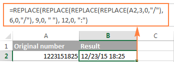
Replacing a string that appears in a different position in each cell
So far, in all the examples we have been dealing with values of a similar nature and have made replacements in the same position in each cell. But real-life tasks are often more complicated than that. In your worksheets, the characters to be replaced may not necessarily appear in the same place in each cell, and therefore you will have to find the position of the first character that should be replaced. The following example will demonstrate what I'm talking about.
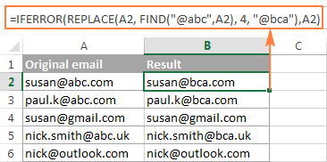
Supposing you have a list of email addressing in column A. And the name of one company has changed from "ABC" to, say, "BCA". So, you have to update all of the clients' email addressing accordingly.
But the problem is that the client names are of different length, and that is why you cannot specify exactly where the company name begins. In other words, you do not know what value to supply in the start_num argument of the Excel REPLACE function. To find it out, use the Excel FIND function to determine the position of the first char in the string "@abc":
=FIND("@abc",A2)
And then, supply the above FIND function in the start_num argument of your REPLACE formula:
=REPLACE(A2, FIND("@abc",A2), 4, "@bca")
Tip. We include "@" in our Excel Find and Replace formula to avoid accidental replacements in the name part of email addresses. Of course, there's a very slim chance that such matches will occur, and still you may want to be on the safe side.
As you see in the following screenshot, the formula has no problem with finding and replacing the old text with the new one. However, if the text string to be replaced is not found, the formula returns the #VALUE! error:
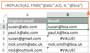
And we want the formula to return the original email address instead of the error. So, let's enclose our FIND & REPLACE formula in the IFERROR function:
=IFERROR(REPLACE(A2, FIND("@abc",A2), 4, "@bca"),A2)
And this improved formula works perfectly, doesn't it?
Another practical application of the REPLACE function is to capitalize the first letter in a cell. Whenever you deal with a list of names, products, and the like, you can use the above-linked formula to change the first letter to UPPERCASE.
Tip. If you want to make the replacements in the original data, an easier way would be using the Excel FIND and REPLACE dialog.
Excel SUBSTITUTE function
The SUBSTITUTE function in Excel replaces one or more instances of a given character or text string with a specified character(s).
The syntax of the Excel SUBSTITUTE function is as follows:
The first three arguments are required and the last one is optional.
- Text - the original text in which you want to substitute characters. Can be supplied as a test string, cell reference, or a result of another formula.
- Old_text - the character(s) you want to replace.
- New_text - the new character(s) to replace old_text with.
- Instance_num - the occurrence of old_text you want to replace. If omitted, every occurrence of the old text will be changed to the new text.
For example, all of the below formulas substitute "1" with "2" in cell A2, but return different results depending on which number you supply in the last argument:
=SUBSTITUTE(A2, "1", "2", 1) - Substitutes the first occurrence of "1" with "2".
=SUBSTITUTE(A2, "1", "2", 2) - Substitutes the second occurrence of "1" with "2".
=SUBSTITUTE(A2, "1", "2") - Substitutes all occurrences of "1" with "2".

In practice, the SUBSTITUTE function is also used for removing unwanted characters from cells. For real-life examples, please see:
Note. The SUBSTITUTE function in Excel is case-sensitive. For example, the following formula replaces all instances of the uppercase "X" with "Y" in cell A2, but it won't replace any instances of the lowercase "x".

Substitute multiple values with a single formula (nested SUBSTITUTE)
As is the case with the Excel REPLACE function, you can nest several SUBSTITUTE functions within a single formula to do several substitutions at a time, i.e. substitute several characters or substrings with a single formula.
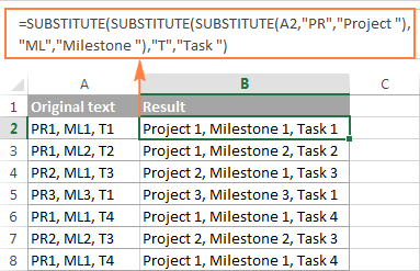
Supposing you have a text string like "PR1, ML1, T1" in cell A2, where "PR" stands for "Project, "ML" stands for "Milestone" and "T" means "Task". What you want is to replace the three codes with full names. To achieve this, you can write 3 different SUBSTITUTE formulas:
=SUBSTITUTE(A2,"PR", "Project ")
=SUBSTITUTE(A2, "ML", "Milestone ")
=SUBSTITUTE(A2, "T", "Task ")
And then nest them into each other:
=SUBSTITUTE(SUBSTITUTE(SUBSTITUTE(A2,"PR","Project "),"ML","Milestone "),"T","Task ")
Notice that we've added a space at the end of each new_text argument for better readability.
To learn other ways to replace multiple values at a time, please see How to do mass find and replace in Excel.
Excel REPLACE vs. Excel SUBSTITUTE
The Excel REPLACE and SUBSTITUTE functions are very similar to each other in that both are designed to swap text strings. The differences between the two functions are as follows:
- SUBSTITUTE replaces one or more instances of a given character or a text string. So, if you know the text to be replaced, use the Excel SUBSTITUTE function.
- REPLACE changes characters in a specified position of a text string. So, if you know the position of the character(s) to be replaced, use the Excel REPLACE function.
- The SUBSTITUTE function in Excel allows adding an optional parameter (instance_num) that specifies which occurrence of old_text should be changed to new_text.
This is how you use the SUBSTITUTE and REPLACE functions in Excel. Hopefully, these examples will prove useful in solving your tasks. I thank you for reading and hope to see on our blog next week!
Download practice workbook
REPLACE and SUBSTITUTE formula examples (.xlsx file)
 by
by
299 comments
How can I replace below:
A1: I need you
to
B1: "I" "need" "you"
Best regards,
Hi! If I understand your task correctly, the following SUBSTITUTE formula should work for you:
=""""&SUBSTITUTE(A1," ",""" """)&""""
Hi!
I used following function to replace a "-" in to 3 places. It works but when already available a "-", then it comes twice in to the same place.
I want skip if available a "-" in B column. Can you please give a solution.
=REPLACE(REPLACE(REPLACE(B2101,7,0,"-"),10,0,"-"),12,0,"-")
E.g.
B2101 C2101
Saman2B3P056 Saman2-B3-P-056
Saman2B2P226 Saman2-B2-P-226
Saman2-B2-P-222 Saman2--B-2--P-222
Saman2-B3-P-011 Saman2--B-3--P-011
Thanks.
Hi! Remove all "-" signs from the text using the SUBSTITUTE function and use that value in your formula. If I understand your task correctly, the formula might look something like this:
=REPLACE(REPLACE(REPLACE(SUBSTITUTE(B2,"-",""),7,0,"-"),10,0,"-"),12,0,"-")
Thank you! Happy Friday! Assalamualaikum!!!
I have a (big) list of prices for items. Some cells have multiple values depending on the pack size of the product:
2 = $20
1 = $35.95, 2 = $57.95, 3 = $71.95
I need to generate the same table but with a 20% increase in price. So, my result table will have:
2 = $24
1 = $43.14, 2 = $69.54, 3 = $86.34
Could you please assist how to do this one using excel? Thanks in advanced.
Hi! If I understand your task correctly, the following tutorial should help: How to calculate percentage in Excel - formula examples.
I have an employer who generates Excel reports from a third-party application, listing numbers as like (for example):
1
11
1743
2
2247
321
The problem with this is that it's quite impossible to sort these numbers in numerical order. In order to solve for this issue, I would like to add "0" or "00" prefix to any of the numbers until they all have the same length. The outcome would have to be:
0001
0011
1743
0002
2247
0321
(which can then be sorted in numerical order)
Is there a way to do this?
Hi! Your problem is that the numbers are written as text, making it impossible to sort them numerically. To solve this, follow the recommended method to convert the text to numbers: How to convert text to number in Excel.
Or you can use text values and these guidelines: How to add leading zeros to text strings. For example:
=REPT("0",4-LEN(A1))&A1
=RIGHT("0000"&A1,4)
Hi.
I have what appears to be a simple request. I'd like a number that appears in a list to be removed if entered elsewhere.
For example, cell A10 contains a small list of numbers like 3 6 7 11 12 17.
Cells A1 - A9 are blank, but if I enter any of these numbers individually into one of these cells that number is removed from the list.
So say I enter "3" in A5, "11" in A2 and "12" in A8 then I'd like A10 to automatically show 6 7 17.
Is it possible?
Thanks
Michael
Hi! You can change the text in cell A10 either manually or by using a VBA macro. If your values will be written in separate cells, you may find this article helpful: How to get a list of unique and distinct values in Excel.
Hi!,
I'm having trouble trying to come up with an excel formula for a macro i've created for the below.
I have a date column which will always the current days date in the below format
28/11/2023
I then have a ref column which needs to be yesterdays date but it includes letters
RT.27.11
So tomorrow for example I will have the date column as 29/11/2023 but im wondering is there a formula that can be used to change AB.27.11 to AB.28.11? I need to keep the Ref letters at the beginning so =Today()-1 isn't an option unless there is a combination I'm unaware of
Apologies if this isn't explained very well I've hit a dead end!
Thanks!
Hi! To combine part of a date with a text string, convert the date to text. For instructions and example formulas, see here: Convert date to text in Excel - TEXT function and no-formula ways.
="RT."&TEXT(TODAY(),"dd.mm")
Hello!
Thanks for this helpful page.
In the screenshot of the example replacing 2014 to 2016, should the formula be
=REPLACE(A24,4,1,"6")
instead of
=REPLACE(A24,4,4,"6") ?
The second formula works, but just because there doesn't happen to be any characters after "4." It seems like the goal is just to replace one character.
Thanks again!
I have file paths of differing lengths and I want to remove the file name so I just have the folder path. So it would always be replacing the last "\" character with a "|" so I could then do a text to columns using the "|" character. I can count the number of times the "\" occurs in the string, in this case 13 times. But can I replace the 13th occurrence of the "\" with "|"?
Change this:
\\pzijasdks28.corp.friend.co.au\shared-fri12\dark\comms - lans\00 archive all\00 finding information\00 archive\2002 comms\campaigns - pre 2002\kisland\mj3k\letter to alan.doc
to this:
\\pzijasdks28.corp.friend.co.au\shared-fri12\dark\comms - lans\00 archive all\00 finding information\00 archive\2002 comms\campaigns - pre 2002\kisland\mj3k|letter to alan.doc
Hi! Please read this manual carefully. In the SUBSTITUTE function, you can specify the character occurrence number to be replaced. Try this formula:
=SUBSTITUTE(A1,"\","|",13)
I have tried to add comma in between First and Last name and to remove Jr. using =SUBSTITUTE(SUBSTITUTE(A1," ",", "),"Jr."," ") but it turned out to be Lemon , , Watermelon (original was Lemon Jr. Watermelon). What formula to help returning this name to be Lemon Watermelon ?
Hi! If I understand your task correctly, try the following formula:
=SUBSTITUTE(A1,"Jr.",", ")
Hi, Can someone help me i have 1000+ entries in which formula is =SUM(ColorCnt(Assir!A1,Assir!AC2:AC110)) i want to replace it with =SUM(Assir!AC2:AC110)) and can i remove colorcnt formula once for all in entire sheet? PLEASE heklp/
Hi! Use the Find&Replace tool to replace or delete text in formulas.Use option "Look in formulas". Read more: How to use Find and Replace in Excel most efficiently.
Hi Can someone help me come up with a formal that removes all the words except for the numbers? I have 1000 plus data and I don't have time to do this one by one. Here are some sample data below, thanks!
Medium Grey 37 Change to 37
Medium Grey 38 Change to 38
Silver 41 Change to 41
Silver 42 Change to 42
Light/Pastel Grey 51 Change to 51
Light/Pastel Grey 52 Change to 51
Hi! We have a special tutorial on this. Please see: How to extract number from string in Excel. I hope it’ll be helpful. If something is still unclear, please feel free to ask.
Hello , can anyone recommend formula or power query way for copy data in a column based on value which can change
example
Cell A2 have name John in it
Cells A3 - A50 have dates
Cell A51 have name Terry in it
Cell A52 - A150 have dates
I want to replace all the dates with names which are above in 10000 rows spreadsheets
any help will be much appreciated
Hello! Excel formula can only change the value in the cell in which it is written. Perhaps you will find a method that works for you in this article: How to find and replace multiple values at once in Excel (bulk replace).
Hello, I'm trying to do a conditional substitution. For example is cell A1 has "John" in it, I want A2 to read "J001", but if cell A1 has "Don" in it, I want cell A2 it to read "D004", etc. Can that be done?
THANK YOU
Hi!
You can change the value of a cell by condition by using the nested IF function. Use these guidelines: Excel Nested IF statements - examples, best practices and alternatives.
=IF(A1="John","J001",IF(A1="Don","D004","")
If you have many conditions, I recommend using the IFS function
=IFS(A1="John","J001",A1="Don","D004")
Imagine if you will that cell A1 has the following content: Abba was a great band.
Cell 2 is supposed to use Replace and/or Substitute to change the six occurrences of a to the replacements in cell 3
Cell 3 has the following: 123456
So cell 2 should come up and look like: 1bb2 w3s 4 gre5t b6nd.
I could probably use Left to slowly strip down A1 into individual characters, run a check, replace if they are an a (or A) to the next in A3 and use left on A3 to slowly reduce it.. but it seems a lot of extra cells when I am already planning a worksheet that should stress test my gaming laptop...
Hi!
Use a nested SUBSTITUTE function
=SUBSTITUTE(SUBSTITUTE(SUBSTITUTE(SUBSTITUTE(SUBSTITUTE(SUBSTITUTE(A1,"a",1,1),"a",2,1),"a",3,1),"a",4,1),"a",5,1),"a",6,1)
I hope this will help.
I created an email from one cell containing first/ last name ie. Ralph M Waters using formula =right(A26,8)&left(a26,1)&lower("@yhospital.com")). this resulted in M WatersR@yhospital.com. I feel as though I've tried every possible formula to include the "_" after the M with no successful results.
Hi I have the texts below in the column A1 to A3, how can convert them to decimals?
E.g.
AFL 1⅛ 03/15/2026 --> AFL 1.125 03/15/2026
AFL 2 ⅞ 10/15/26 --> AFL 2.875 10/15/26
AFL 4 ¾ 01/15/49 --> AFL 4.75 01/15/49
Just to clarify, my goal is to automate this. If I have a list of 300 similar text, I want to drag the solution down to apply to other cells too.
The formula: =REPLACE(A5,5,2,"1.125") gives me the output AFL 1.125 03/15/2026 Corp, but the parameter "1.125" would be to manual.
I appreciate any hint or tips!
Hi!
In your text, ⅛ is a single character. It cannot be converted into a number.
Thank you Alexander!
If I have the following formula...
=+('\\Fileserv\sharedfiles\Safety Reports\OSHA Recordkeeping\[OSHA Reporting Hours.xlsx]2022'!$AR4*200000)/('\\Fileserv\sharedfiles\Safety Reports\OSHA Recordkeeping\[OSHA Reporting Hours.xlsx]2022'!$AS$4)
How can I replace the "2022" in the formula to "2023" easily?
I have a formula that is pages long just like the one above and I need to change approximately 40 "2022's" with "2023".
Hello!
To replace part of a formula on a worksheet, use the Excel Find and Replace tool. Set "Look in" option to "Formulas". For more information, please visit: How to use Find and Replace in Excel most efficiently.
Hi, how can replace BO and 80 to B0 and replace the O and I with 0 and 1. Examples are with * hope you can help me. TYIA
BOIOIOI*
B010102
8010103*
B010104
B010105
B010106
8010107*
8010108*
B010109
BOIOIIO*
BOIOIII*
8010112*
B010113
B010114
B010115
8010116*
8010117*
B010118
Hi!
Have you tried the ways described in this blog post? If they don't work for you, then please tell me which formulas you used. I’ll try to suggest a solution.
Please Help!
Lets say A1 = 8x12 as a text. I need to replace "x" with " x " . Respectively I need to add space between x and number on each side.
So I would write SUBSTITUTE(A1,"x"," x "), but it works only on some occasions while it does not work on others the only difference between occasions is the numbers on either side of x (like 40x70 or 100x30 and so on).
Can anyone of you please explain how to fix this so it works on every instance or suggest an alternative that works indefinitely?
Thanks in advance!
Hi!
I don't understand why the formula doesn't work for you. She works for me. Explain the problem.
Hi , May I get help regarding issue mentioned. Thanks a lot.
If i update C2 with text, A2 will be updated
If i delete text in C2, key in D2, A2 will be updated with text from D2
If i delete text in C2/D2, key in E2, A2 will be updated with text from E2
My concern here is , I want to reflect A2 as latest one whenever there is input in C/D or E.
My case here, input to C/D or E will be one after another, where A2 to reflect with latest info from C/D or E.
Thanks
My current formula used in A2 is =IF(C3="C","Cyellow",(IF(D3="D","Dyellow",(IF(E3="E","Eyellow","")))))
Hello!
To find the last non-blank cell in a range, use one of the formulas below:
=INDEX(C2:E2,,COUNTA(C2:E2))
=LOOKUP(2, 1/(C2:E2<>""), C2:E2)
Read more in this guide: Look up a value in the last non-blank cell.
I just want to say this was incredibly useful!, that nested replace is a game changer, thank you so much.
Hi,
I got following string in one cell:
_1x111xAx0_22x222xAAx00_333x333xAAAx000_4x444xAAAAx0000_55x555xAAAAAx00000_(etc.)
As you can see there are segments divided by _
I need a formula that will change every first x in each segment to /
Result should be:
_1/111xAx0_22/222xAAx00_333/333xAAAx000_4/444xAAAAx0000_55/555xAAAAAx00000_(etc.)
Any ideas?
Thanks!
@Sreco
hmmm...not a formula, but you could use:
Data > Text to Columns > Delimited > Other (_)
to turn that one column of cells into a multiple column array,
then use the substitution formula to swap the first instance of x in each cell
then use the concat formula to rejoin them, or just use
=Sheet!A1&"_"&Sheet!B1&"_"&etc...
maybe with a switch function that counts the number of rows and modifies the above formula
if there aren't a consistent number of "_" in each string...
pretty manual, but less manual than doing it by hand.
I'm sure there's a better option, especially if using VBA.
@Sreco
Actually, a better way...(tested, it works, and copy/paste scale-able):
Sheet1!A1=your string
Sheet2!A1=1
Sheet2!B1=FIND("x",Sheet1!$A1,FIND("_",Sheet1!$A1,Sheet2!A1))
Sheet2!C1=FIND("x",Sheet1!$A1,FIND("_",Sheet1!$A1,Sheet2!B1))
etc...
Sheet3!A1=Sheet1!$A1
Sheet3!B1=REPLACE(Sheet3!A1,FIND("x",Sheet3!A1,Sheet2!B1),1,"/")
Sheet3!C1=REPLACE(Sheet3!B1,FIND("x",Sheet3!B1,Sheet2!C1),1,"/")
etc...
when using the substitute formula, how can get the numbers to display correctly. this is the formula i am using:
=SUBSTITUTE(SUBSTITUTE(SUBSTITUTE($D$2:$D$5000,"1","item1"),"3","item3"),"13","item13")
what it should do is look for instances of a number in column D, and put a word in place of the number.
so if d:3 has a "1" in it the return is "item1". the problem i have is that when "13" is the number the formula returns both 1, and 3, values: "item1item3".
how can i get this formula to accurately display "1", "3" and "13"?
Hello!
The formula below will do the trick for you:
=SUBSTITUTE(SUBSTITUTE(SUBSTITUTE($D$2:$D$5000,"1","item1"),"3","item3"), "item1item3","item13")
Hi,
Please help, I need to replace text from " HD " to " A " for example if the range from A2:AD2 the sum of text of " HD " is >2 so here I need to replace the " HD " under in same range A2:AD2 except over and above 2 " HD" cases.
Hi!
An Excel formula cannot change values in a range of cells. You need to use a VBA macro.
How to delete/hide specific words in a cell and just show what I want to show?
Example:
On Cell G2, this is the text: "Here is my task for today, hoping to finish it asap."
I want to just show this word in another cell: "today"
Hi I'm hoping you can help me ...
I have the following Exchange Powershell command and I would like the values in quotes to be equal to details stored in another cell on the same row.
Set-DistributionGroup -Identity "value1" -Name "value2" -DisplayName "value3" -IgnoreNamingPolicy
This Powershell command would be located in Cell F2. I would like the result to replace value1 with contents of Cell A2 and replace value2 & value3 with contents of Cell B2. I am then wanting to copy the working formula for around 700 rows each time replacing the "value?" entries with Cell A and Cell B of the corresponding row e.g. copying formula to F3 would populate with Cells A3 & B3 and so forth.
Cheers,
Duncan
Hi!
If I understand correctly, you want to concatenate text and cell values. Here is a detailed guide with examples: CONCATENATE in Excel: combine text strings, cells and columns.
"Set-DistributionGroup -Identity " & A2 & " -Name " & B2 & " -DisplayName " & B2 & " -IgnoreNamingPolicy"
Hope this is what you need.
Hi Alexander,
Thanks so much for replying and pointing me in the right direction ... took me only 5 minutes o get it working I just needed an "=" at the front of the example you provided ... see below.
="Set-DistributionGroup -Identity " & A3 & " -Name " & B3 & " -DisplayName " & B3 & " -IgnoreNamingPolicy"
Trying to see if I can replace a value (number) from on cell with 2 different letters depending on the value. So if returned value from formula is 1 in A3 then BL is displayed in A4 (the new cell for this new formula). If value is 2 then OR is displayed. 3 then GR is displayed and so on up to 12? I know that you can do single letters for a given number but need 2 letters to differentiate in further letters. Thank you in advance.
Hi!
Based on your description, it is hard to completely understand your task. However, I’ll try to guess and offer you use CHOOSE function.
=CHOOSE(A3,"BL","OR","GR",..........)
I hope it’ll be helpful.
how to replace the text in the same row but in multiple columns in a workbook??
As in my workbook, one column is Code Second is Catagory which is the same I need to replace the category column with another code no. i can replace in 30 sheets it's difficult
Hi!
An Excel formula can only change the value of the cell in which it is written. For your task, you need to write VBA code
1 year 9 months = 1.9
can someone help with the above results?
=REPLACE(E2, 1, 79,)
=SUBSTITUTE(F2,CHAR(9),"")
How can i combine these formulas?
Hi!
I am not sure I fully understand what you mean. Your formulas refer to different cells. You can combine them using the IF function. But you didn't specify the condition for this. Your question is not entirely clear, please specify.
exmple
row c5 2020 41566565
if found in row c5 such cell change in r5521
its cell complete change
how can change data such type
Hi!
I am not sure I fully understand what you mean.
Hi, very nice thing you got here going on.
I've encountered a little problem with the substitute function. Assuming this is the formula I use in my reference cell S2:
=SUM(IF(AY2=AZ2;1;0)+IF(AY3=AZ3;1;0)
And then I use in another cell:
=SUBSTITUTE(SUBSTITUTE(S2;"AY";"BG"),"AZ","BH")
to keep the formula the same, but to have every AY substituted by BG, and every AZ by BH. However, I can't get it to work. How come?
Thank you in advance.
BTW I did notice that in your examples, in the examples, ', ' (a comma) is used, whereas I use ';' (a point comma). But the point comma is automatically used by the excel I use itself, so that can't be the issue I guess.
Hello!
You cannot change the formula with another formula. You can use the INDIRECT function to create links.
I have a conversion table. I would like Excel to automatically change the numbers when I type them in.
For example;
if I type in 176123456789, I'd like it to change the numbers to 176xxxxx6789
A part of the conversion table looks like this:
176xxxxx6789 after i type the number inside
and it continues. is this a possibility?
If your number length is fixed then you can use below formula.
=SUBSTITUTE(A2,MID(A2,4,5),"xxxx")
I have a conversion table. I would like Excel to automatically change the numbers when I type them in.
For example;
if I type in 10.25, I'd like it to change the numbers after the decimal point to .4... final number should look like 10.4
A part of the conversion table looks like this:
.10-.15=.2 (.10 THROUGH .15 is .2)
.16-.21=.3
.22-.27=.4
and it continues. is this a possibility?
Thank you for your consideration.
Hi!
You cannot change the number that you wrote in a cell using an Excel function. You need to use VBA macro. In the adjacent cell, you can use the IF function to get the number according to your conditions.
I hope I answered your question. If you have any other questions, please don’t hesitate to ask.
i want to enter numbers that will be translated in text (pre-defined for each number)
for example , if i enter "0" in a cell and press enter, it will be translated as "negative"
1 = positive
2 = good ,etc
Hi!
Use a VBA macro. But you cannot enter ordinary numbers.
Hi ATTA:
You can use the following formula:
=IF(F5=0, "Negative", IF(F5=1, "Positive", IF(F5=2, "Good", "False")))
Hello,
How i can replace below .
11.11111.1111 to 11.11111-1111
the last dot should be dash.
Best regards
Hello!
You can use this formula:
=SUBSTITUTE(A1,".","-",LEN(A1)-LEN(SUBSTITUTE(A1,".","")))
I recommend reading this guide: How to count characters in Excel
Hi,
Sir,
Thank you very much.
Best regards
Hi Shajith,
You can also use the following formula:
=REPLACE(B20, 9, 1, "-")
I used "SUBSTITUTE" function to remove commas from a number but now I can't add the number I got with other numbers since it is now stored as a text I guess. Any solution for this??
Hi!
If you are talking about a decimal point, then use the rounding functions. If this is not what you want, please explain in more detail.
Give an example of the source data and the expected result.
For some reason, when I try to use the SUBSTITUTE() function in VBA code, I get an error that says "Sub or Function not defined" when running the macro, with the "Substitute" portion of the code highlighted, as if VBA can't find that function. Am I missing a reference package or something? I thought Substitute() was part of the base Excel install. Why isn't VBA find that function??? Replace() it can find, and everything else I've tried, just not Substitute().
BTW, if I type it directly into a cell as a formula, it works OK there. Just not in VBA for some reason.
Is there any possibility of adding specific texts to allocated number values please?
e.g.
0 = None
1 = Tea
2 = Cocoa
3 = Coffee
Thank you in advance for any suggestions.
Hi!
Based on your description, it is hard to completely understand your task. However, I’ll try to guess and offer you the following formula:
=CHOOSE(B1+1,B1&"None", B1&"Tea", B1&"Cocoa", B1&"Coffee")
If this is not what you wanted, please describe the problem in more detail.
Is there any possibility of adding specific texts to allocated number values please?
e.g.
0 = Not Yet Achieved
1 = Pass
2 = Merit
3 = Distinction
Thank you in advance for any suggestions.
hi Cam,
You can use the following formula:
=IF(F9=0, "Not Yet Achieved", IF(F9=1, "Pass", IF(F9=2, "Merit", IF(F9=3, "Distinction", "False"))))
where, F9 is the first cell number with the number 0.