The article looks at how to quickly remove part of text from Excel cells using formulas and inbuilt features.
In this tutorial, we will look at the most common cases of removing characters in Excel. Want to delete specific text from multiple cells? Or maybe strip the first or last character in a string? Or perhaps remove only a specific occurrence of a given character? Whatever your task is, you will find more than one solution for it!
How to remove specific character in Excel
If your goal is to eradicate a certain character from Excel cells, there are two easy ways to do it - the Find & Replace tool and a formula.
Remove character from multiple cells using Find and Replace
Bearing in mind that removing a character is nothing else than replacing it with nothing, you can leverage Excel's Find and Replace feature to accomplish the task.
- Select a range of cells where you want to remove a specific character.
- Press Ctrl + H to open the Find and Replace dialog.
- In the Find what box, type the character.
- Leave the Replace with box empty.
- Click Replace all.
As an example, here's how you can delete the # symbol from cells A2 through A6.
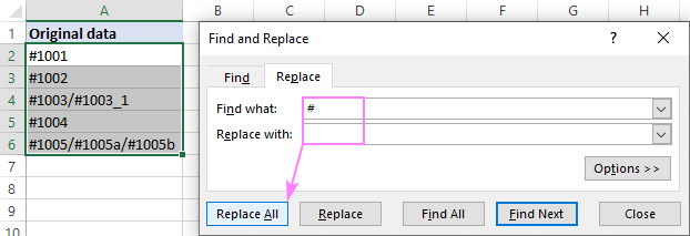
As the result, the hash symbol is removed from all of the selected cells at once, and a pop-up dialog informs you how many replacements have been made:

Tips and notes:
- This method deletes characters directly in your source data. If the result is different from what you expected, press Ctrl + Z to undo the change and get your original data back.
- If you are dealing with alphabetical characters where the letter case matters, click Options to expand the Find and Replace dialog, and then tick the Match case box to perform case-sensitive search.
Remove certain character from string using a formula
To eliminate a specific character from any position is a string, use this generic SUBSTITUTE formula:
In our case, the formula takes this form:
=SUBSTITUTE(A2, "#", "")
Basically, what the formula does is that it processes the string in A2 and replaces each hash symbol (#) with an empty string ("").
Enter the above formula in B2, copy it down through B6, and you will get this result:
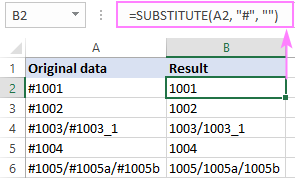
Please pay attention that SUBSTITUTE always returns a text string, even if the result contains only numbers like in cells B2 and B3 (notice the default left alignment typical for text values).
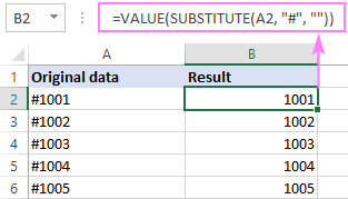
If you want the result to be a number, then wrap the above formula in the VALUE function like this:
=VALUE(SUBSTITUTE(A2, "#", ""))
Or you can perform some math operation that does not change the original value, say add 0 or multiply by 1:
=SUBSTITUTE(A2, "#", "")*1
Delete multiple characters at once
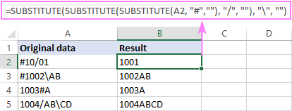
To remove multiple characters with one formula, simply nest SUBSTITUTE functions one into another.
For example, to get rid of a hash symbol (#), forward slash (/) and backslash (\), here's the formula to use:
=SUBSTITUTE(SUBSTITUTE(SUBSTITUTE(A2, "#",""), "/", ""), "\", "")
Tips and notes:
- The SUBSTITUTE function is case-sensitive, please keep that in mind when working with letters.
- If you'd like to have the results as values independent on the original strings, use the Paste special - Values option to replace formulas with their values.
- In situation when there are many different characters to remove, a custom LAMBDA-defined RemoveChars function is a lot more convenient to use.
How to remove certain text from Excel cell
The two methods we used for removing a single character can handle a sequence of characters equally well.
Delete text from multiple cells
To remove specific text from each cell in a selected range, press Ctrl + H to display the Find and Replace dialog, and then:
- Enter the unwanted text in the Find what box.
- Leave the Replace with box blank.
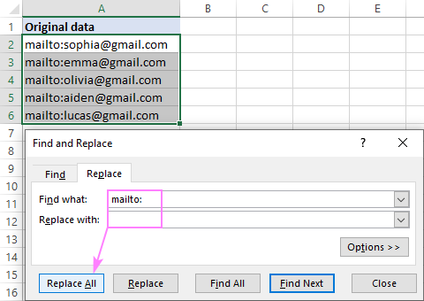
Clicking the Replace All button will do all the replacements in one go:

Remove certain text from cell using a formula
To remove part of a text string, you again use the SUBSTITUTE function in its basic form:
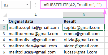
For example, to delete the substring "mailto:" from cell A2, the formula is:
=SUBSTITUTE(A2, "mailto:", "")
This formula goes to B2, and then you drag it down across as many rows as needed:
How to remove Nth instance of a specific character
In situation when you want to delete a certain occurrence of a particular character, define the last optional argument of the SUBSTITUTE function. In the generic formula below, instance_num determines which instance of the specified character should be replaced with an empty string:
For example:
To eradicate the 1st slash in A2, your formula is:
=SUBSTITUTE(A2, "/", "", 1)
To strip the 2nd slash character, the formula is:
=SUBSTITUTE(A2, "/", "", 2)

How to remove first character
To remove the first character from the left side of a string, you can use one of the following formulas. Both do the same thing, but in different ways.
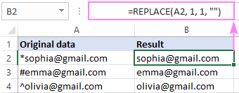
Translated into a human language, the formula says: in the specified cell, take 1 character (num_chars) from the 1st position (start_num), and replace it with an empty string ("").
Here, we subtract 1 character from the total length of the string, which is calculated by the LEN function. The difference is passed to RIGHT for it to extract that number of characters from the end.
For instance, to remove the first character from A2, the formulas go as follows:
=REPLACE(A2, 1, 1, "")
=RIGHT(A2, LEN(A2) - 1)
The screenshot below shows the REPLACE formula. The RIGHT LEN formula will deliver exactly the same results.
To delete any n characters from the beginning of a string, please see How to remove characters from left in Excel.
How to remove last character
To strip off the last character from the end of a string, the formula is:
The logic is similar to the RIGHT LEN formula from the previous example:
You subtract 1 from the total cell length and serve the difference to the LEFT function, so it can pull that many characters from the beginning of the string.
For instance, you can remove the last character from A2 using this formula:
=LEFT(A2, LEN(A2) - 1)

To delete any n characters from the end of a string, please see How to remove characters from right in Excel.
Remove text after a specific character
To delete everything after a given character, the generic formula is:
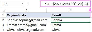
The logic is quite simple: the SEARCH function calculates the position of the specified character and passes it over to the LEFT function, which brings the corresponding number of characters from the beginning. Not to output the delimiter itself, we subtract 1 from the SEARCH result.
For example, to remove text after a colon (:), the formula in B2 is:
=LEFT(A2, SEARCH(":", A2) -1)
For more formula examples, please see Delete text before or after a certain character.
How to remove spaces before and after text in Excel
In text processors such as Microsoft Word, a whitespace before text is sometimes added intentionally to create a balanced and elegant flow for the reader's eye. In spreadsheets programs, leading and trailing spaces may creep unnoticed and cause a lot of problems. Luckily, Microsoft Excel has a special function, named TRIM, to delete extra spaces.
The formula to remove excess spaces from cells is as simple as this:
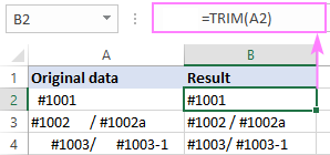
=TRIM(A2)
Where A2 is your original text string.
As you can see in the image below, it deletes all spaces before text, after text and between words/substrings except for a single space character.
If this simple formula does not work for you, then most likely there are some non-breaking spaces or non-printing characters in your worksheet.
To get rid of them, convert non-breaking spaces into regular spaces with the help of SUBSTITUTE:
SUBSTITUTE(A2, CHAR(160), " ")
Where 160 is the code number of a non-breaking space character ( ).
Additionally, use the CLEAN function to eliminate non-printable characters:
CLEAN(SUBSTITUTE(A2, CHAR(160), " "))
Nest the above construction in the TRIM function, and you'll get a perfect formula to remove spaces before/after text as well as non-breaking spaces and non-printing characters:
=TRIM(CLEAN(SUBSTITUTE(A2, CHAR(160), " ")))
For more information, please see How to remove spaces in Excel.
Remove characters in Excel with Flash Fill
In simple scenarios, Excel's Flash Fill can do you a favor and remove characters or part of text automatically based on the pattern that you provide.
Let's say you have a name and email address in one cell separated by a comma. You want to remove everything after the comma (including the comma itself). To have it done, carry out these steps:
- Insert a blank column to the right of your source data.
- In the first cell of a newly added column, type the value you want to keep (name in our case).
- Start typing the value in the next cell. As soon as Excel determines the pattern, it will show a preview of data to be filled in the below cells following the same pattern.
- Press the Enter key to accept the preview.
Done!
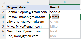
Note. If Excel is unable to recognize a pattern in your data, fill in a couple more cells manually to provide more examples. Also, make sure Flash Fill is enabled in your Excel. If it still does not work, then you'll have to resort to some other method.
Special tools to remove characters or text in Excel
This final section presents our own solutions for removing text from Excel cells. If you love finding simple ways to handle complex challenges, you'll enjoy the handy tools included with Ultimate Suite.
On the Ablebits Data tab, in the Text group, there are three options for removing characters from Excel cells:
- Specific characters and substrings
- Characters in a certain position
- Duplicate characters
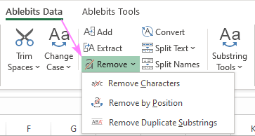
To delete a specific character or substring from selected cells, proceed in this way:
- Click Remove > Remove Characters.
- Select the option best suited to your needs.
- Check or uncheck the Case-sensitive box.
- Hit Remove.
Below are a few examples that cover the most typical scenarios.
Remove specific character
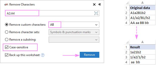
To remove a particular character(s) from multiple cells at once, select Remove custom characters.
As an example, we are deleting all occurrences of the uppercase letters A and B from the range A2:A4:
Delete a predefined character set
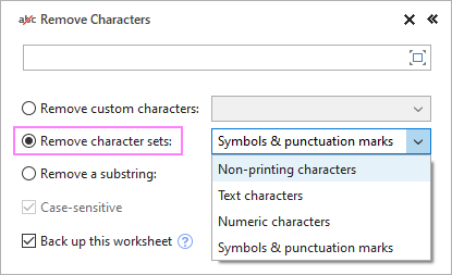
To remove a certain set of characters, select Remove character sets, and then choose one of the following options:
- Non-printing characters - strips off any of the first 32 characters in the 7-bit ASCII set (code values 0 through 31) including a tab character, line break, and so on.
- Text characters - removes text and keeps numbers.
- Numeric characters - deletes numbers from alphanumeric strings.
- Symbols & punctuation marks - removes special symbols and punctuation marks such as a period, question mark, exclamation point, comma, etc.
Remove part of text
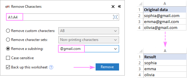
To delete part of a string, choose the Remove a substring option.
For example, to extract usernames from Gmail addresses, we are removing the "@gmail.com" substring:
That's how to remove text and characters from Excel cells. I thank you for reading and look forward to seeing you on our blog next week!
Available downloads
Remove characters in Excel - examples (.xlsm file)
Ultimate Suite - evaluation version (.exe file)
 by
by
93 comments
Hello,
I am trying to separate or remove just the date on one cell tried textafter,textsplit still doesn't work
example in one cell value includes date and time ==> "4/1/2024 05:00 AM" - I just want to remove the date or move it to another cell and remain just the time.
Please help
Thank you
Hello Navin!
Unfortunately, I don't know what result you want: "05:00 AM", "05:00" or 05:00 as time.
To extract the text between the second and third spaces "05:00", you can use these guidelines: Split string by comma, semicolon, slash, dash or other delimiter.
The formula might look like this:
=MID(A2, SEARCH(" ",A2) + 1, SEARCH(" ",A2,SEARCH(" ",A2)+2) - SEARCH(" ",A2) - 1)
With this formula, you extract the time as text.
With the TEXTBEFORE and TEXTAFTER functions, you can get the time as text:
=TEXTAFTER(A2," ",1)
or
=TEXTBEFORE(TEXTAFTER(A2," ",1)," ")
To get the time from the text, you can use the TIMEVALUE function:
=TIMEVALUE(TEXTBEFORE(TEXTAFTER(A2," ",1)," "))
=TIMEVALUE(MID(A2,SEARCH(" ",A2)+1,SEARCH(" ",A2,SEARCH(" ",A2)+2)-SEARCH(" ",A2)-1))
If the format of this text matches your system date and time settings, you can convert the text to date and time using a mathematical operation and then get the time value:
=(MOD(--A2,1))
Set the desired time format in the formula cell.
Dear Team,
Basic Data:
1.Blocks Work
2.Plasting Work
3.Scaffolding Work
4.Chiping Work
5.Barbending Work
6.Shuttering Work
7.Cleaning Work
8.Water Curing
9.Welding Work & Cutting Work.
Results:
Blocks Work, Plasting Work, Scaffolding Work, Chiping Work, Barbending Work, Shuttering Work, Cleaning Work, Water Curing and Welding Work & Cutting Work.
Is this possible ?
Hello! Merge all values into one text string using the TEXTJOIN function. The following tutorial should help: TEXTJOIN function in Excel to merge text from multiple cells.
TEXTJOIN(", ",TRUE,A1:A5)
Remove all dots or other unwanted characters using the SUBSTITUTE function.
SUBSTITUTE(TEXTJOIN(", ",TRUE,A1:A5),".","")
Remove all numbers from the text string using this instruction: How to remove numbers from text string in Excel.
=TEXTJOIN("", TRUE, IF(ISERROR(MID(SUBSTITUTE(TEXTJOIN(", ",TRUE,A1:A5),".",""), SEQUENCE(LEN(SUBSTITUTE(TEXTJOIN(", ",TRUE,A1:A5),".",""))), 1) *1), MID(SUBSTITUTE(TEXTJOIN(", ",TRUE,A1:A5),".",""), SEQUENCE(LEN(SUBSTITUTE(TEXTJOIN(", ",TRUE,A1:A5),".",""))), 1), ""))
Hope this is what you need.
Hello Sir,
I have an inventory file with item description cell. I have to import this file to new pos. New pos requires description limit to 30 characters max. I do have items that has more than 30. I would like to cut the description of the items that has more than 30 characters to 30. Is there a way to remove few letters from the item description in the middle. I like to keep the first and last 15 characters and remove few fr0m the middle to make it total of 30.
EXMP. Bombay sapphire London Dry Gin 750 ml. This has 37 total characters I want to reduce to 30 by removing 7 from the middle and leave first and last 15 as is.
is there any formula for this? I have quite a big list. what is the best way to do this form multiple items.
is there a function where you can use it to find more than 30 characters in a cell and reduce to 30 by keeping first and last 15.
Thanks
Count the number of characters in a text string using the LEN function. Use the LEFT function to get the first 15 characters. Use the RIGHT function to get the last 15 characters. Combine text strings using the & operator. Please try the following formula:
=IF(LEN(A1)>30,LEFT(A1,15)&RIGHT(A1,15),A1)
Thanks for quick reply.
Formula works perfectly for the cell that has more than 30 characters.
But if the cell has less than 30 character it add more txt to make it 30 characters.
EXMP: GATORADE 32 OZ it changes to "GATORADE 32 OZGATORADE 32 OZ"
HOT MIX SNACKS > "HOT MIX SNACKSHOT MIX SNACKS"
is there a function that this only work for more than 30 characters? I would just copy and paste this for all the cells and whichever cell has more than 30 characters, formula applies and if its 30 or less no change being done to that cell.
Thanks again for your help.
Hi! To avoid wasting my time and yours, it would be nice if you described the problem in full. Also, your example result is 28 characters, not 30. You can paste the text from the cell twice and get the first 30 characters. For example:
=IF(LEN(A1)>30,LEFT(A1,15)&RIGHT(A1,15),LEFT(A1&A1,30))
Thanks for Reply and let me explain in detail.
here are the text in a 2 different cell. Let's say cell is B2 and other is B3 and so on.
(B2) - Bombay Sapphire London Dry Gin 750 ML - (total 37 letters including spaces)
(B3) - Water 1 LT - (10 characters)
So I like to reduce the B2 cell characters from 37 to 30 and for this your first formula work perfect. The formula reduces the character from the middle and brings it down to 30.
But If I use same formula for the cell B3, here is the outcome of applying the formula. (Water 1LTWater 1LT)
Because I have more than 1000 cells with those kind of description where some cells would be more than 30 letters and some would under 30.
I can not pick and apply formula individually because I have more than 1000 cells.
I was asking that if there was a way to use the formula that would only reduce if the cell has more than 30 letters and does not make any changes to the cell that has 30 or less.
So I would like to copy the formula to the all the cells and formula only works for the cell with more than 30 letters.
Thank You again for your time.
The first formula I recommended meets those conditions. In the second comment you wanted different.
I require excel formula to eliminate the numerical value following each backslash \ in order to obtain the desired output as presented below.
D:\Documents\3.0 Mexic\3.1 Vega\3.1.8 O&M\3.1.8.5 ESG\3.1.8.5.3 ESG C\3.1.8.5.3.2 NATUR\3.1.8.5.3.2.2 GUAJI\3.1.8.5.3.2.2.2 01_Pr\3.1.8.5.3.2.2.2.3 Anexo\3.1.8.5.3.2.2.2.3.2 Visit\3.1.8.5.3.2.2.2.3.2.2 P.S\3.1.8.5.3.2.2.2.3.2.2.2 PROGR
output as below
D:\Documents\Mexic\Vega\O&M\ESG\ESG C\NATUR\GUAJI\01_Pr\Anexo\Visit\P.S\PROGR
Hi! To remove all numbers and dots from the text, you can use the recommendations from the paragraph above: Delete multiple characters at once.
=SUBSTITUTE(SUBSTITUTE(SUBSTITUTE(SUBSTITUTE(SUBSTITUTE(SUBSTITUTE(SUBSTITUTE(SUBSTITUTE(SUBSTITUTE(SUBSTITUTE(SUBSTITUTE(SUBSTITUTE(A1," ",""),".",""),0,""),9,""),8,""),7,""),6,""),5,""),4,""),3,""),2,""),1,"")
However, you won't get the desired result as you don't want to remove all numbers and not all spaces and dots.
I am looking for away to extract the date in each string.
The names are like these:
7_dfgdfh_20190425_8.JPG
4_fhdrd_20190425_10.JPG
524_ID289_sdf_sdg_sdf_20160607_(3).JPG
473_ID4_sdf_sdg_20200405_(13).JPG
7754_ID785_346I_20230809_(101).JPG
Result:
20190425
20190425
20160607
20200405
20230809
I think RegExpExtract() is the answer because in each name there ist his pattern "_20******_",but Ican't figure it out.
Any help? :D
Hi! To extract numbers from text using a pattern, please take a look at this article: Regex to extract strings in Excel (one or all matches). I believe the following formula will help you solve your task:
=SUBSTITUTE(RegExpExtract(A1, "_20(.*?)_", 1),"_","")
I am looking for a way to remove the last question mark from a offer url whenever there will be any ? Mark at the end of the offer url
Hi! Unfortunately, this information is not enough to give you any advice. Maybe this guide will be helpful: Remove last character in Excel.
000001 - I need to replace the first zero in the string to a 1
Hi! Find the position of the first "0" using the SEARCH function and replace it with a "1" using the REPLACE function. Try this formula:
=REPLACE(A1,SEARCH("0",A1),1,1)
i am looking for a way to remove the "-" from the below format
for example 3-A & vice versa
its a working file with more than 10000 line items with multiple formats from this i need to change only the "-" between an alphabet & number and vice versa. remaining "-" i need to keep, for example "-" between the numbers. Will you please give me a solution for this.
Nested substitute worked very well for me. Thank you
Hi, how to remove and separate into separate column.
Before
No.K/P : 123456-12-1234 / 123456
After
123456-12-1234 123456
I want to remove everything after the - that is after the word Mississauga how do I do that?
Hi! The formulas below will do the trick for you:
=LEFT(A1,SEARCH(C1,A1)-1)&C1
or
=TEXTBEFORE(A1,C1)&C1
For more information, please visit: Excel TEXTBEFORE function - extract text before character (delimiter).
hi sir alexander,
i have 123400000567890 in A1, i want to replace zeros with "-" like this: 1234-567890
sometimes zeros changes like this, 432100000009876 and i want to replace it with 4321-9876
or sometimes like this, 789000000012345 and replace it with 7890-12345
number in A1 is always 15 digits and i want to replace consecutive zeros after the 4 digits with "-"
is it possible?? thanks in advance
To replace characters in a string by a pattern, you can use regular expressions and the custom RegExpReplace function.
For example,
=LEFT(A1,4)&RegExpReplace(MID(A1,5,20), "0{3,10}", "-")
We extract the first 4 characters from the text. In the rest of the text, starting from the fifth character, the RegExpReplace function looks for a group of zeros from 3 to 10 and replaces them with "-".
For more information, please visit: Excel Regex to find and replace strings using regular expressions. I hope my advice will help you solve your task.
Thank you sir Alexander, it helps a lot. It works like a charm! And also thanks to Bill Finchy for tracing the syntax error.
Thank you So So So much. It helped me a lot.
Original data
40 Test1
5 Test2
139 Test3
Result:
Test1
Test2
Test3
Original
6.1 moving
2.2 NDT
6.3.3 refurbishment
6.4.1 documenting
4.5.1.6 documenting2
Result:
Moving
Process
refurbishment
documenting
documenting2
I spent hours to find solution, your help is greatly appreciated.
Hi! To remove text before the first space, you can use the SEARCH function and REPLACE function :
=REPLACE(A2,1,SEARCH(" ",A2),"")
If have a line like this " @Raja @rani @john @will you are so sweeet!. so I want to delete the name after @ with @ sign. Be clear I want to delete the name with @. Means output will be only " you are so sweeet!". How I delete all the name at a time so only meaningful sentence will output.?
Hi!
To find all substrings in the text that match the pattern and remove them, the custom function RegExpReplace is used. It is used to replace the text. To remove substrings matching the pattern, use an empty string ("") to replace them.
You can find the examples and detailed instructions here: Excel Regex to remove certain characters or text from strings.
@.*?\s\b - pattern
=RegExpReplace(A1, "@.*?\s\b", "", 1) - formula
I recommend paying attention to the Regex tools. You can find, extract, remove, or replace strings that match a regex pattern you enter. It is available as a part of our Ultimate Suite for Excel that you can install in a trial mode and check how it works for free.
Hi,
I have a question with the string, provide a dummy as below:
A AA AAA AAAA ICPxxdays xx/xx/xxxx CC123456 BBBBB
And I wish to get the text only CC123456.
Hi!
You can extract characters from text with the custom function RegExpExtract.
To extract 2 letters and 6 digits from anywhere in the text, try the formula:
=RegExpExtract(A1, "..\d{6}")
You can find the examples and detailed instructions here: How to extract substrings in Excel using regular expressions (Regex).
You can find, extract, remove, or replace strings that match a regex pattern using Regex Tools. It is available as a part of our Ultimate Suite for Excel that you can install in a trial mode and check how it works for free.
I have series of strings
MM36-1-APPLE
MM36-1-GRAPE
MM38-2-APPLE
MM2-1-ORANGE
.....
The result would be:
APPLE
GRAPE
APPLE
ORANGE
...
i want remove
MM36-1-
MM36-1-
MM38-2-
MM2-1-
These values in bulk i have more than 3000+data like this
Note: Text to columns not for me"
Please answer my query thanks in advance
Hi!
You can find the examples and detailed instructions here: How to remove text before the last occurrence of a character.
Try this formula:
=TRIM(RIGHT(A2, LEN(A2) - FIND("#", SUBSTITUTE(A2, "-", "#", LEN(A2) - LEN(SUBSTITUTE(A2, "-",""))))))
Hello Alex and albeit team, do you mind helping me write a formula based on these sets of data?
so the original data would be: Social Media Group(socialmediagroup.com)
and the result I'm expecting: socialmediagroup.com
I used this formula
=RIGHT(C3;SEARCH("(";C3)-1)
even tried the ones with "LEN", I cannot seem to find the solution.
thank you
Hello!
To extract text between two characters, you can use this article's recommendations: Extract text between two characters in Excel.
=MID(A1,SEARCH("(",A1)+1,SEARCH(")",A1)-SEARCH("(",A1)-1)
or
=TEXTBEFORE(TEXTAFTER(A1, "("), ")")
This should solve your task.
tried this from above samples and seems to have worked as well...
=SUBSTITUTE((SUBSTITUTE(C15,"Social Media Group(","")),")","")
Dear Concern,
I have a list of data as below around 9000 row. From each of row I want to remove all text after "M" (3000M). How can I do this please advise. Thanks.
Eco Poly; 100% Premium Poly Poly Corespun; Tex-60; Tkt-50; 3000M (44049)
Best regrads,
Mahbub Ar Rashid
Dhaka, Bangladesh
Hello!
Find a text string using the SEARCH function and use the LEFT function.
=LEFT(A1,SEARCH("3000M",A1)+4)
A2 = Party's Name
B2 = Address with pin
A2 - Aaditi Krushi Seva Kendra-Lingali
B2 - Aaditi Krushi Seva Kendra-Lingali & his full address
I have data in 2000 row, I want in C2 only address without party's Name.
Can you help me
Hi!
Based on your description, it is hard to completely understand your task. However, I’ll try to guess and offer you the following formula:
=SUBSTITUTE(B2,A2,"")
You can learn more about SUBSTITUTE function in Excel in this article on our blog.
A2 B2
Party's Name Address with pin
Aaditi Krushi Seva Kendra-Lingali "Aaditi Krushi Seva Kendra-Lingali, (full address)
Aaditya Krushi Seva Kendra-Nitrud Aaditya Krushi Seva Kendra-Nitrud (full address)
Aae Pedkae K.S.Kendra, Ashte Aae Pedkae K.S.Kendra, Ashte (full address)
have data in Large number of row, I want in C2 only address without party's Name.
Can you help me
Hi!
I can't guess what you want to extract from the text.
How can I clean this:
102095
105679-02
100794_D
CBT106145
Result:
102095-00
105679-02
100794-00
106145-00
I want to get rid of the letter and the underscore only.
Is there a way to remove three words from an excel spreadsheet. the three words needing to be removed from each cell are all of different lengths but are all separated by a space
Hello!
Try to use these recommendations: Regex to remove certain characters or text in Excel.
Hi Alexander,
I have name ABC Travels and Tours in A1 and in A2 i have used following formula =TRIM(LEFT(A1,FIND("^",SUBSTITUTE(A1," ","^",2)&"^"))) to arrive at the following result: ABC Travels.
Now instead of Travels just require Travel so what will be the formula that i can use.
Regards/Irfan
Hi!
If I understand correctly, the LEFT function should extract 2 less characters.
=TRIM(LEFT(A1,FIND("^",SUBSTITUTE(A1," ","^",2)&"^")-2))
Dear Alexander,
Thank you for your reply, I tried the formula you suggested, However it gives the result with one character less for the words in second place.
Since I have data in thousand of rows and i only want the result with one less character of particular word i.e Travels and formula should give me the result as Travel.
Irfan
Hi!
The formula returns: ABC Travel. If I understand correctly, you wanted this result.
Hello!
Yes Correct.
Hello Alexander,
I have figured out the following formula.
=TRIM(LEFT(A1,FIND("^",SUBSTITUTE(SUBSTITUTE(A1," ","^",2),"TRAVELS"," ")&"^")))
will above formula be consistent and work smoothly?
Regards/Irfan
=TRIM(LEFT(A1,FIND("^",SUBSTITUTE(SUBSTITUTE(A1," ","^",2),"TRAVELS"," ")&"^")))
Note: After Travels in inverted commas i have kept 5 spaces
Hello :)
I need to remove the last digits in a string of text eg “Thomas Andrew jeffery 5555” the length of number at the end may vary
Hello!
Please check the formula below, it should work for you:
=LEFT(A1,SEARCH("#",SUBSTITUTE(A1," ","#",LEN(A1)-LEN(SUBSTITUTE(A1," ",""))))-1)
For more information, please read: How to split text in Excel using formulas.
To extract all the text before a specific character, you can use the Excel TEXTBEFORE function.
=TEXTBEFORE(A1," ",LEN(A1)-LEN(SUBSTITUTE(A1," ","")))
I hope my advice will help you solve your task.
Hello, I want to remove all the characters to the right of the date sequence.
The date sequence is written as Year,Month , Day.
All I want after its done is for the data in each column to remain.
Example of unmodified cells:
20110904_Acts1_1-3.mp3
20110911_Acts1_4-8.mp3
20110918_Acts2_1-4.mp3
How I want it to look afterward:
20110904
20110911
20110918
What im ultimately trying to do is have the Date in one Column and what comes after the date in another column. However the person who started it this was listen the data and the title in the same string.
Ultimately it would look like this:
COLUMN 1 COLUMN2
20110904 Acts1_1-3.mp3
20110911 Acts1_4-8.mp3
20110918 Acts2_1-4.mp3
Hello!
You can manually split a string with the Text to Columns feature.
You can split text using formulas, as described in this article.
=LEFT(A2, SEARCH("_",A2)-1)
=RIGHT(A2,LEN(A2)-SEARCH("_",A2))
You can also use the new Excel functions TEXTBEFORE and TEXTAFTER to get the string before and after the delimiter.
=TEXTBEFORE(A2,"_",1)
=TEXTAFTER(A2,"_",1)
This should solve your task.
Hi,
I have the following text on a cell: Matthew Stafford\StafMa00
and I need to only have Last Name, First Name (Stafford, Matthew)
Thanks so much!
Hello!
Excel substring functions to extract text from cell
=LEFT(A1,SEARCH("\",A1)-1)
You can also use the new function TEXTBEFORE:
=TEXTBEFORE(A1,"\")
Hi,
I need to adjust a sequence of numbers for an efficient pivot sheet, right now I manually remove the additional characters and it’s extremely time consuming. An example is below:
Ping: James Carpenter 38754689 15
Ping: James Carpenter 38763532 15
Ping: Janet Jackson 47627645 15
Ping: Ming Lee 47657374 15
Ping: Seymour Leften 36875267 15
I just need “Ping: (first/last name)” or “Ping: James Carpenter…
What formula could I use to simplify each cell in order to save time on my pivot sheets?
Thanks!
VR
Hello!
If your data has a common pattern, then extract all characters up to the third space. Replace the third space with the SUBSTITUTE function. Find its position using the SEARCH function.
Please try the following formula:
=LEFT(A1,SEARCH("#",SUBSTITUTE(A1," ","#",3),3))
Hi, hope you can help me.
I have a sheet that contains cells with data I do not want. Such as:
"Save"
"View profile"
"Add Phil Nock to selection"
etc...
They all have a pattern, in the sense that the cells I do not want all have a pattern throughout the sheet, either containing a whole word in a cell like "add" or with text that follows the common word "add Phil Nock..."
I have a list of common words that are found after i have sorted my list to satisfaction, but have no clue how to "Find" a word in a cell, and "remove" who whole cell if that word is found, whether it is in whole or in part "add" or "add Phil..."
Hi!
Try using the Excel Find and Select tool. Try to use the recommendations described in this guide: Excel Find and Replace with wildcards. To remove, use replace with nothing.
Hope you’ll find this information helpful.
i have case about IP
118.98.100.117
118.98.101.1
118.98.101.108
118.98.101.12
118.98.101.123
i need to remove the last character after "." and add with "0/24"
the result should be 118.98.101.0/24
Hello!
To remove text after a specific character try this formula -
=LEFT(A1,SEARCH("#", SUBSTITUTE(A1,".","#",LEN(A1)- LEN(SUBSTITUTE(A1,".","")))))&"0/24"
For more information, please visit: Excel substring functions to extract text from cell.
Thank you so much... you just saved me many hours... :-)
Sir i want to remove text into columns from every cells but i can't find any solution .It is very difficult for me .
following text is to be extract:
Saadan Hospital (Johar Town) Rs. 1,500Available todayRs. 1,500 Iqra Medical Complex (Ext.) (Johar Town) Rs. 2,000Available tomorrowRs. 2,000 Zainab Medical Centre (Wapda Town) (Wapda Town) Rs. 1,500Available todayRs. 1,500 Online Video Consultation (Online) Rs. 1,200Available todayRs. 1,200 Tahir Hospital (Raiwind Road) Rs. 1,500 Schedule: N/ARs. 1,500
Sir i want to extract in following type
Saadan Hospital (Johar Town), Iqra Medical Complex (Ext.) (Johar Town), Zainab Medical Centre (Wapda Town), Tahir Hospital (Raiwind Road)
Thanks M Mushahid
Hi!
Split text into columns as described in this instruction. Then merge cells that contain the information you want.
I have series of strings
UNUNK1986
UNJUN1986
01JUN1986
in the same column
I want to remove "UNUNK" from UNUNK1986 and "UN" from UNJUN1986 and need to apply text join in next column.
Thank you
Varun
Hi!
Please re-check at the article above since it covers your case.
Hi I have a string of reviews mined from a review site like this:
Trish Mar 30 2022 9:09 pm
This series moved me to tears quite a few times. BRILLIANT acting by all actors and actresses involved. Thank You for your hard work. CHEERS!
How do I remove the name and date/time for all 1518 rows?
Hello!
Use the SEARCH function to find the position of the first space and line break. Extract text at these positions and concatenate strings.
Please try the following formula:
=LEFT(A1,SEARCH(" ",A1))&MID(A1,SEARCH(CHAR(10),A1),200)
Vehicle number
1st case
GJ5AB9998 need to add 0 before 5
Need to see like GJ05AB9998
2nd case
GJ05AB998
Need add 0 before 998
Hi!
Your data does not have any pattern. Determine the position of the desired character using the SEARCH function. Split text with substring functions. Use the & operator to insert "0".
=LEFT(A1,SEARCH("5",A1)-1)&"0"&MID(A1,SEARCH("5",A1),50)
Hi,
I have the following string in a cell:
ME.SA.02.14 (MSG)
I need a formula that would help me get the following string ME.SA.02 (MSG)
Hi!
To remove a string from text, use the recommendations from the article above, as well as this instruction: Using REPLACE and SUBSTITUTE functions in Excel - formula examples
=REPLACE(A1,9,3,"")
I hope this will help.
Hello,
I have a string in a cell 0108997237110515211116342164401725022810TMC22009
I want to extract 21111634216440 from it and paste that at the back after 9
is this possible ?
Hi!
What pattern do you want to extract numbers from text?
For this example, you can use the MID function
=A1&MID(A1,17,14)
Hi guys,
I was wondering if the CTRL+H option can be done automatically.
I mean, when I scan an article on Excel there is always a #00 after the code (ex: BDC#00). Is there a VBA to remove automatically the #00 on range B8:B20 after to press Enter and keep only "BDC"?
Thank you a lot for your help.
Patrick.
Hi!
You can change the value in the current cell either manually or using a VBA macro. To get the desired value in another cell, use text functions. For example, the LEFT function
=LEFT(B8,3)
Hi Alex,
thanks for your reply. However and due to another VBA, cells cannot have any functions. It has to be only with a VBA code such as
Private Sub Workbook_SheetChange(ByVal Sh As Object, ByVal Target As Range)
Do you have any idea how to build this VBA`?
Thanks you so much.
Pat.
thank you!
I'm trying to combine a RIGHT/LEN to remove the first X# of characters, which is fine, but I'm trying to leverage a vlookup to get the value to remove. I can nest the VLOOKUP in the RIGHT formula, but can't seem to figure out how to add the LEN after that lookup and reference the value the VLOOKUP is returning. Any suggestions without doing 2 columns of lookups?
Logically, what I want it something like this =RIGHT(VLOOKUP.....),LEN(*result of the vlookup),-10
Hello!
So that I can help you, write an example of the source data and explain what result you want to get.
This is very helpful. God bless you ?
Well done!!
Is it possible to remove strings of text from other cells if they repeat in a previous cell? I am trying to do this with any random partial duplicates. I am trying keep the first occurrence of a string but delete that string from other cells.
For example, I want to delete any strings that repeat and are more than 2 characters long.
abc
def
ghi
jkl
abdgj
adetyk
Since "ab" is in the first cell and also the 5th cell, is it possible to delete the "ab" in the 5th cell? So the first cell will still be "abc" but the 5th will change to "dgi".
"de" also repeats in 2nd and 6th cell, "de" to only remain in the 2nd cell but be deleted in the 6th cell. 2nd cell will remain "def" but the 6th cell will change to "atyk".
Is this possible? I have been looking it up for hours but can't seem to find a solution.
Thank you very much.
Hi!
A formula may only modify the value of the cell into which it is written. Your task cannot be solved using ordinary Excel formulas. You need to use the VBA macro.
This helped me solve CSV files where the broker Binance had spammed USDT and commas in every line!
try this in MS Word's find and replace:
Find: space^p
Replace with: ^p
Replace All , several times until trailing spaces (or space) at the end deleted
^p is a special character for replaces Enter (paragraph mark)
for another purposes, look at More - Special
I'm looking for a way to remove the last character (generally a space) at the end of a cell in WORD 2019.
This space is generally included when I copy a spreadsheet from EXCEL to WORD.
I can not find a way for the WORD 2019 to find the Cell Mark at the end of a cell in Word. If I can do this, I can concatenate the character + the cell mark and type ^H to call the find and replace window.
Best Regards,
Julio Borges
Rio de Janeiro - Brasil