The tutorial explains the uses of ROUND, ROUNDUP, ROUNDDOWN, FLOOR, CEILING, MROUND and other Excel rounding functions and provides formula examples to round decimal numbers to integers or to a certain number of decimal places, extract a fractional part, round to nearest 5, 10 or 100, and more.
In some situations when you don't need an exact answer, rounding is a useful skill to use. In plain English, to round a number is to eliminate the least significant digits, making it simpler but keeping close to the original value. In other words, rounding lets you get an approximate number with the desired level of accuracy.
In everyday life, rounding is commonly used to make numbers easier to estimate, communicate or work with. For instance, you can use rounding to make long decimal numbers shorter to report the results of complex calculations or round off currency values.
Many different ways of rounding exist, such as rounding to integer, rounding to a specified increment, rounding to simple fractions, and so on. And Microsoft Excel provides a handful of functions to handle different rounding types. Below, you will find a quick overview of the major round functions and well as formula examples that demonstrate how to use those functions on the real-life data in your worksheets.
Excel rounding by changing the cell format
If you want to round numbers solely for presentations purposes, then you can just change the number of displayed decimal places without changing the underlying value. The fastest way is to use the Increase Decimal or Decrease Decimal command on the Home tab in the Number group:
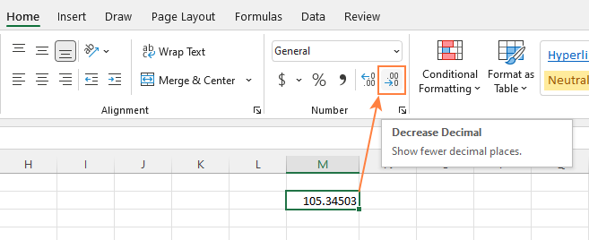
Or you can change the cell's format by performing these steps:
- Select the cell with the number(s) you want to round.
- Open the Format Cells dialog by pressing Ctrl + 1 or right click the cell(s) and choose Format Cells... from the context menu.
- In the Format Cells window, switch to either Number or Currency tab, and type the number of decimal places you want to display in the Decimal places box. A preview of the rounded number will immediately show up under Sample.
- Click the OK button to save the changes and close the Format Cells dialog.

Important note! This method changes the display format without changing the actual value stored in a cell. If you refer to that cell in any formulas, the original non-round value will be used in all calculations.
Excel functions to round numbers
Unlike formatting options that change only the display value, Excel round functions alter the actual value in a cell.
Below you will find a list of functions specially designed for performing different types of rounding in Excel.
- ROUND - round the number to the specified number of digits.
- ROUNDUP - round the number upward to the specified number of digits.
- ROUNDDOWN - round the number downward to the specified number of digits.
- MROUND - rounds the number upward or downward to the specified multiple.
- FLOOR - round the number down to the specified multiple.
- CEILING - round the number up to the specified multiple.
- INT - round the number down to the nearest integer.
- TRUNC - truncate the number to a specified number of decimal places.
- EVEN - round the number up to the nearest even integer.
- ODD - round the number up to the nearest odd integer.
Excel ROUND function
ROUND is the major rounding function in Excel that rounds a numeric value to a specified number of digits.
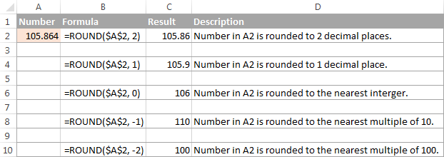
Syntax: ROUND(number, num_digits)
Number - any real number you want to round. This can be a number, reference to a cell containing the number or a formula-driven value.
Num_digits - the number of digits to round the number to. You can supply a positive or negative value in this argument:
- If num_digits is greater than 0, the number is rounded to the specified number of decimal places.
For example
=ROUND(15.55,1)rounds 15.55 to 15.6. - If num_digits is less than 0, all decimal places are removed and the number is rounded to the left of the decimal point (to the nearest ten, hundred, thousand, etc.).
For example
=ROUND(15.55,-1)rounds 15.55 to the nearest 10 and returns 20 as the result. - If num_digits equals 0, the number is rounded to the nearest integer (no decimal places).
For example
=ROUND(15.55,0)rounds 15.55 to 16.
The Excel ROUND function follows the general math rules for rounding, where the number to the right of the rounding digit determines whether the number is rounded upwards or downwards.
Rounding digit is the last significant digit retained once the number is rounded, and it gets changed depending on whether the digit that follows it is greater or less than 5:
- If the digit to the right of the rounding digit is 0, 1, 2, 3, or 4, the rounding digit is not changed, and the number is said to be rounded down.
- If the rounding digit is followed by 5, 6, 7, 8, or 9, the rounding digit is increased by one, and the number is rounded up.
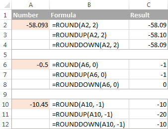
The following screenshot demonstrates a few ROUND formula examples:
Excel ROUNDUP function
The ROUNDUP function rounds the number upward (away from 0) to a specified number of digits.
Syntax: ROUNDUP(number, num_digits)
Number - the number to be rounded up.
Num_digits - the number of digits you want to round the number to. You can supply both positive and negative numbers in this argument, and it works like num_digits of the ROUND function discussed above, except that a number is always rounded upward.

Excel ROUNDDOWN function
The ROUNDDOWN function in Excel does the opposite of what ROUNDUP does, i.e. rounds a number down, toward zero.
Syntax: ROUNDDOWN(number, num_digits)
Number - the number to be rounded down.
Num_digits - the number of digits you want to round the number to. It works like the num_digits argument of the ROUND function, except that a number is always rounded downward.
The following screenshot demonstrates the ROUNDDOWN function in action.

Excel MROUND function
The MROUND function in Excel rounds a given number up or down to the specified multiple.
Syntax: MROUND(number, multiple)
Number - the value you want to round.
Multiple - the multiple to which you want to round the number.
For example, the below formula rounds 7 to the nearest multiple of 2 and returns 8 as the result:
=MROUND(7, 2)
Whether the last remaining digit is rounded up (away from 0) or down (towards 0) depends on the remainder from dividing the number argument by the multiple argument:
- If the remainder is equal to or greater than half the value of the multiple argument, Excel MROUND rounds the last digit up.
- If the remainder is less than half the value of the multiple argument, the last digit is rounded down.
The MROUND function comes in handy, say, for rounding prices to the nearest nickel (5 cents) or a dime (10 cents) to avoid dealing with pennies as change.

And, it is really indispensable when it comes to rounding times to a desired interval. For example, to round time to the nearest 5 or 10 minutes, just supply "0:05" or "0:10" for the multiple, like this:
=MROUND(A2,"0:05") or =MROUND(A2,"0:10")
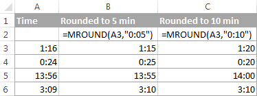
Note. The MROUND function returns the #NUM! error when its arguments have different signs. For example, both of the formulas =MROUND(3, -2) and =MROUND(-5, 2) result in the NUM error.
Excel FLOOR function
The FLOOR function in Excel is used to round a given number down, to the nearest multiple of a specified significance.
Syntax: FLOOR(number, significance)
Number - the number you want to round.
Significance - the multiple to which you wish to round the number.
For example, =FLOOR(2.5, 2) rounds 2.5 down to the nearest multiple of 2, which is 2.
The Excel FLOOR function performs rounding based on the following rules:
- If the number and significance arguments are positive, the number is rounded down, toward zero, as in rows 2 and 10 in the screenshot below.
- If number is positive and significance is negative, the FLOOR function returns the #NUM error, as in row 4.
- If number is negative and significance is positive, the value is rounded down, away from zero, as in row 6.
- If number and significance are negative, the number is rounded up, toward zero, as in row 8.
- If number is an exact multiple of the significance argument, no rounding takes place.
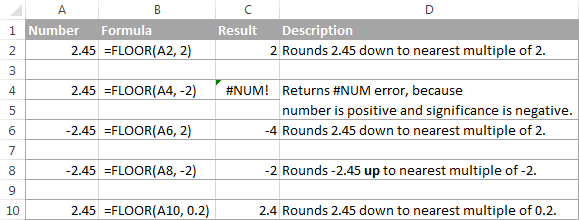
Note. In Excel 2003 & 2007, the number and significance arguments must have the same sign, either positive or negative, otherwise an error is returned. In newer Excel versions, the FLOOR function has been improved, so in Excel 2010, 2013 and 2016 it can handle a negative number and positive significance.
Excel CEILING function
The CEILING function in Excel rounds a given number up, to the nearest multiple of significance. It has the same syntax as the FLOOR function.
Syntax: CEILING(number, significance)
Number - the number you want to round.
Significance - the multiple to which you want to round the number.
For instance, the formula =CEILING(2.5, 2) rounds 2.5 up to the nearest multiple of 2, which is 4.
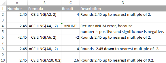
The Excel CEILING function works based on the rounding rules similar to FLOOR's, except that it generally rounds up, away from 0.
- If both the number and significance arguments are positive, the number is rounded up, as in rows 2 and 10 in the screenshot below.
- If number is positive and significance is negative, the CEILING function returns the #NUM error, as in row 4.
- If number is negative and significance is positive, the value is rounded up, towards zero, as in row 6.
- If number and significance are negative, the value is rounded down, as in row 8.
Excel INT function
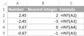
The INT function rounds a number down to the nearest integer.
Of all Excel round functions, INT is probably the easiest one to use, because it requires only one argument.
Syntax: INT(number)
Number - the number you want to round down to the nearest integer.
Positive numbers are rounded toward 0 while negative numbers are rounded away from 0. For example, =INT(1.5) returns 1 and =INT(-1.5) returns -2.
Excel TRUNC function
The TRUNC function truncates a given numeric value to a specified number of decimal places.
Syntax: TRUNC(number, [num_digits])
- Number - any real number that you want to truncate.
- Num_digits - an optional argument that defines the precision of the truncation, i.e. the number of decimal places to truncate the number to. If omitted, the number is truncated to an integer (zero decimal places).
The Excel TRUNC function adheres to the following rounding rules:
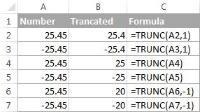
- If num_digits is positive, the number is truncated to the specified number of digits to the right of the decimal point.
- If num_digits is negative, the number is truncated to the specified number of digits to the left of the decimal point.
- If num_digits is 0 or omitted, it rounds the number to an integer. In this case, the TRUNC function works similarly to INT in that both return integers. However, TRUNC simply removes the factional part, while INT rounds a number down to the nearest integer.For example,
=TRUNC(-2.4)returns -2, while=INT(-2.4)returns -3 because it's the lower integer. For more info, please see Rounding to integer example.
The following screenshot demonstrates the TRUNC function in action:
Excel ODD and EVEN functions
These are two more functions provided by Excel for rounding a specified number to an integer.
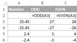
ODD(number) rounds up to the nearest odd integer.
EVEN(number) rounds up to the nearest even integer.
- In both functions, number is any real number that you want to round.
- If number is non-numeric, the functions return the #VALUE! error.
- If number is negative, it is rounded away from zero.
The ODD and EVEN functions may prove useful when you are processing items that come in pairs.
For example:
=ODD(2.4) returns 3
=ODD(-2.4) returns -3
=EVEN(2.4) returns 4
=EVEN(-2.4) returns -4
Using rounding formulas in Excel
As you see, there exist a variety of functions to round off numbers in Excel depending on the particular purpose. The following examples will hopefully give you some clues on how to use Excel rounding formulas based on your criteria.
How to round decimals in Excel to a certain number of places
Depending on the situation, you may want to round decimals up, down or based on math rounding rules:
ROUNDUP function - always rounds the decimal upward.
ROUNDDOWN function - always rounds the decimal downward.
ROUND - rounds up if the rounding digit is followed by the digit equal to or greater than 5, otherwise rounds down.
As an example, lets round the decimal numbers in column A to 2 decimal places. In the first argument (number), you enter a reference to the cell containing the number, and in the second argument (num_digits) you specify the number of decimal places you want to keep.
=ROUNDUP(A2, 2) - rounds the number in A2 upward, to two decimal places.
=ROUNDDOWN(A2, 2) - rounds the number in A2 downward, to two decimal places.
=ROUND(A2, 2) - rounds the number in A2 to 2 decimal places, upward or downward, depending on whether the 3rd decimal digit is greater or less than 5.

Rounding negative numbers (ROUND, ROUNDDOWN, ROUNDUP)
When it comes to rounding a negative number, the results returned by the Excel round functions, may seem to flout logic :)
When the ROUNDUP function applies to negative numbers, they are said to be rounded up, even though they actually decrease in value. For example, the result of =ROUNDUP(-0.5, 0) is -1, as in row 7 in the screenshot below.
The ROUNDDOWN function is known to round numbers downward, though negative numbers may increase in value. For example, the formula =ROUNDDOWN(-0.5, 0) returns 0, as in row 8 in the screenshot below.
In fact, the rounding logic with regard to negative numbers is very simple. Whenever you use the ROUND, ROUNDDOWN or ROUNDUP function in Excel on a negative number, that number is first converted to its absolute value (without the minus sign), then the rounding operation occurs, and then the negative sign is re-applied to the result.
How to extract a decimal part of a number
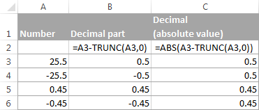
If you want to extract a fractional part of a decimal number, you can use the TRUNC function to truncate the decimal places and then subtract that integer from the original decimal number.
=A2 - TRUNC(A2,0)
As demonstrated in the screenshot below, the formula in column B works perfectly both for positive and negative numbers. However, if you'd rather get an absolute value (decimal part without the minus sign), then wrap the formula in the ABS function:
=ABS(A2 - TRUNC(A2,0))
How to round a decimal to an integer in Excel
As is the case with rounding to a certain number of decimal places, there is a handful of functions for rounding a fractional number to an integer.
ROUNDUP
To round up to nearest integer, use an Excel ROUNDUP formula with num_digits set to 0. For example =ROUNDUP(5.5, 0) rounds decimal 5.5 to 6.
INT or ROUNDDOW
To round down to nearest whole number, use either INT or ROUNDDOW with num_digits set to 0. For example both of the following formulas round 5.5 to 5:
=ROUNDOWN(5.5, 0)
=INT(5.5)
For negative decimals, however, the INT and ROUNDDOWN functions yield different results - INT rounds negative decimals away from 0, while ROUNDDOWN toward 0:
=ROUNDOWN(-5.5, 0) returns -5.
=INT(-5.5) returns -6.
TRUNC
To remove the factional part without changing the integer part, use the TRUNC formula with the second argument (num_digits) omitted or set to 0. For example, =TRUNC(5.5) truncates the decimal part (.5) and returns the integer part (5).
ODD or EVEN
To round a decimal up to the nearest odd integer, use the ODD function:
=ODD(5.5) returns 7.
To round a decimal up to the nearest even integer, use the EVEN function:
=EVEN(5.5) returns 6.

Round to nearest 0.5
Microsoft Excel provides 3 functions that let you round numbers to nearest half, more precisely to the nearest multiple of 0.5. Which one to use depends on your rounding criteria.
- To round a number down to nearest 0.5, use the FLOOR function, for example
=FLOOR(A2, 0.5). - To round a number up to nearest 0.5, use the CEILING function, for example
=CEILING(A2, 0.5). - To round a number up or down to nearest 0.5, use the MROUND function, e.g.
=MROUND(A2, 0.5). Whether MROUND rounds the number up or down depends on the remainder from dividing the number by multiple. If the remainder is equal to or greater than half the value of multiple, the number is rounded upward, otherwise downward.

As you see, the MROUND function can be used for rounding positive values only, when applied to negative numbers, it returns the #NUM error.
Round to nearest 5 / 10 / 100 / 1000
Rounding to nearest five, ten, hundred or thousand is done in the same manner as rounding to 0.5 discussed in the previous example.
Round to nearest 5
Supposing that the number you want to round to closest 5 resides in cell A2, you can use on of the following formulas:
- To round a number down to nearest 5:
=FLOOR(A2, 5) - To round a number up to nearest 5:
=CEILING(A2, 5) - To round a number up or down to nearest 5:
=MROUND(A2, 5)

Round to nearest 10
To round your numbers to nearest ten, supply 10 in the second argument of the rounding functions:
- To round a number down to nearest 10:
=FLOOR(A2, 10) - To round a number up to nearest 10:
=CEILING(A2, 10) - To round a number up or down to nearest 10:
=MROUND(A2, 10)

Round to nearest 100
Rounding to a hundred is done in the same way, except that you enter 100 in the second argument:
- To round a number down to nearest 100:
=FLOOR(A2, 100) - To round a number up to nearest 100:
=CEILING(A2, 100) - To round a number up or down to nearest 100
=MROUND(A2, 100)

Round to nearest 1000
To round a value in cell A2 to the nearest thousand, use of the following formulas:
- To round a number down to nearest 1000:
=FLOOR(A2, 1000) - To round a number up to nearest 1000:
=CEILING(A2, 1000) - To round a number up or down to nearest 1000
=MROUND(A2, 1000)

The same techniques can be used for rounding numbers to other multiples. For example, you can round the prices to the nearest nickel (multiple of 0.05), lengths to the nearest inch (multiple of 1/12), or minutes to the nearest second (multiple of 1/60). Speaking of time, and do you know how to convert it to nearest hour or closest 5 or 10 minutes? If you don't, you will find the answers in the next section :)
Rounding time in Excel
There may be many situations when you need to round time values. And again, you can use different rounding functions depending on your purpose.
Example 1. How to round time to nearest hour in Excel
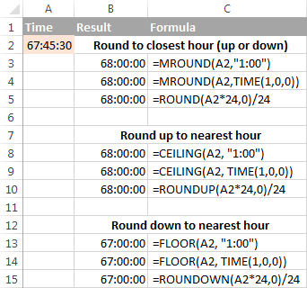
With times located in column A, you can use one of the following functions to round time to nearest hour:
- To round time to closest hour (up or down) - MROUND or ROUND.
=MROUND(A1,"1:00")=MROUND(A1, TIME(1,0,0))=ROUND(A1*24,0)/24 - To round up time to nearest hour - ROUNDUP or CEILING.
=CEILING(A1, "1:00")=CEILING(A1, TIME(1,0,0))=ROUNDUP(A1*24,0)/24 - To round down time to nearest hour - ROUNDDOWN or FLOOR.
=FLOOR(A1, "1:00")=FLOOR(A1, TIME(1,0,0))=ROUNDDOWN(A1*24,0)/24
In the ROUND, ROUNDUP and ROUNDDOWN formulas, you multiply the time value by 24 (number of hours in a day) to convert a serial number representing the time to hours. Then you use one of the rounding functions to round the decimal value to an integer, and then divide it by 24 to change the returned value back to the time format.
If your timestamps include date values, then use the INT or TRUNC function to extract dates (in the internal Excel system, dates and times are stored as serial numbers, the integer part representing a date and fractional part representing time). And then, use the formulas described above but subtract the date value. For example:
=MROUND(A1,"1:00") - INT(A1)
=MROUND(A1,"1:00") - TRUNC(A1)
The following screenshot demonstrates other formulas:
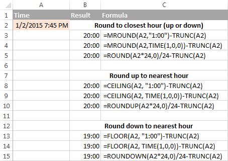
Note. For the results to display correctly, remember to apply the Time format to your cells.
Example 2. Rounding time to nearest 5, 10, 15, etc. minutes
In case you want to round times in your Excel sheet to five or ten minutes, or to the closest quarter-hour, you can use the same rounding techniques as demonstrated above, but replace "1 hour" with the desired number of minutes in the formulas.
For example, to round the time in A1 to the closest 10 minutes, use one of the following functions:
- To round time to closest 10 minutes (up or down):
=MROUND(A1,"0:10")=MROUND(A1, TIME(0,10,0)) - To round up time to nearest 10 min:
=CEILING(A1, "0:10")=CEILING(A1, TIME(0,10,0)) - To round down time to nearest 10 min:
=FLOOR(A1, "0:10")=FLOOR(A1, TIME(0,10,0))

If you know (or can calculate) what portion of a day is constituted by a certain number of minutes, then you won't have problems using the ROUND, ROUNDUP and ROUNDOWN functions as well.
For example, knowing that 15 minutes, is 1/96th of a day, you can use one of the following formulas to round the time in A1 to the nearest quarter-hour.
- To round time to closest 15 minutes (up or down):
=ROUND(A1*96,0)/96 - To round up time to nearest 15 min:
=ROUNDUP(A1*96,0)/96 - To round down time to nearest 15 min:
=ROUNDDOWN(A1*96,0)/96
This is how you perform rounding in Excel. Hopefully, now you know how, among all those round functions, chose the one best suited for your needs.
 by
by
368 comments
If i want to roundup or down for example
If 2nd decimal was 0 2 4 then 3rd decimal was 5 below i want to retain the 2nd decimal to original value for example
1.445
2nd decimal was 4
3rd decimal was 5 below
=1.44
I tried
On cell 2
=Cell1-trunc(cell1)
On cell3
=Mid(cell2,5,1)
On cell4
=If (cell3<5,roundup(cell1,2),rounddown(cell1,2))
But it doesnt work can anyone help thanks in advance
Hi! If I understand the question correctly, you can extract the last digit of the number using the RIGHT function, and if it is "5", round down. Use the IF formula to select rounding by condition. For example:
=IF(RIGHT(A1,1)="5",ROUNDDOWN(A1,2),ROUND(A1,2))
hi, can you help
if
0.01-1.3 = 1
1.31 - 2.3 = 2
2.31 - 3.3 = 3
etc
Hi! Use the IF function to set the value by condition. You can find the examples and detailed instructions here: Nested IF in Excel – formula with multiple conditions.
Very informativr and great site ever and newer I seen. thanks
Sulute to the Team and Developer.
Thanks once again.
How i can remove the 0 from a big number that is being rounded up example ( 12,990,000 ) need to remove the 0
Hi! Unfortunately, I don't really understand what you want to do: round a number or remove zeros from the text. You can remove zeros from a number written as text using the SUBSTITUTE function.
=SUBSTITUTE(A1,"0","")
You can also write a number in thousands using a custom number format "#,##0,". Read more: Custom Excel number format.
Please edit the following chunk:
"functions and well as formula examples that".
Hi , I would like to help with the below.
I am using the below sum
=SUM(D2:K2)*0.095 the result shows 42.40 but when I use that cell to do onwards calculation, it is using the extracted number of 42.39565
How do I stop this or have the cell really round to 42.40 not 42.39565
Thank you
Hi! Use the rounding functions you see in the article above. For example:
=ROUND(SUM(D2:K2)*0.095,2)
Hi good morning, I essentially want to roundUP the displayed figure, similar to what was explained with the increasing/decreasing decimal points. The cells that I'm rounding up are pulling from each other in a table going horizontally across. I tried using the RoundUp feature, but the figure that it's pulling from is the rounded figure, rather than the actual value. Example below:
Actual values
8.04 --> 8.04/1.5 = 5.36 --> 5.36*100/40 = 13.4 --> 13.4*100/40= 33.5
Desired values
9 --> 6 --> 14 --> 34
RoundUp values
9 --> 6 --> 15 --> 38
As it goes further across, the difference between the desired value and roundup value goes further apart. I applied the formula into the roundup function ie =ROUNDUP(H34/1.5,0) {With H34 being the cell representing 8.04} etc. but because it's pulling the rounded number at each stage, the number just gets higher.
Can you guide me to my desired values please? Thanking you in advance. Have a good one.
Hi! Unfortunately, I don't really see how I can help here. If you calculate 6*100/40, you can't get a result of 14.
Yeah, I was hoping there was a way to calculate using the actual values. Therefore, instead of 6*100/40, it uses the initial 5.36, to result in 5.36*100/40, becoming 13.4 and the shown values would be 6 and 14 respectively. Only work-around I see is an additional table with actual values and it would RoundUp the figures on that table instead of itself. Was hoping to avoid that but I'll do it if it's necessary. Thanking you in any case for your response. Have a blessed day.
Hi! Try using the original values rather than the rounded result. For example:
=(8.04/1.5)*100/40
Yeah, but because the number I'm pulling from is the cell itself. Not sure how to link it to the original value rather than the rounded one. The original cell value changes based on other factors so it's essentially x/1.5, 8.04 was just an example, therefore can't be a fixed value. The only way I'm thinking to be able to get it done is a separate table where all the actual values are calculated and I RoundUp my intended results from that rather than the formulated cells.
How do I round it to this result?
≤0.25 = 0
≥0.26 = 0.5
≤0.75 = 0.5
≤0.76 = 1
≥1.25 = 1
≥1.26 = 1.5
Hi! Round the number twice using the FLOOR and CEILING functions as described in the article above:
=FLOOR(CEILING(A1,0.25),0.5)
Hi,
I understand how to use MROUND but is there a way to incorporate it into a cell that already has a formula and have it round the results of the formula in that same cell? For instance I have a cell, let's say cell M32, with the following simple formula: =(E32*E$6/12)+(G32*K$6/12)+(I32*E$7/12)+(K32*K$7/12) . This cell, (M32), produces a number (happens to be a currency figure, for example 5,416.67). I am trying to have this cell (M32) not only calculate the formula but then to round the results of the formula to 25. I know "work arounds", like simply doing a second column producing the rounded number next to the cell with the number produced by the formula but I do not want multiple unnecessary columns. I know this following formula won't work as it refers to itself but intuitively let's say my formula cell is in cell M32 that I also want rounded as stated. Using my above formula, contained in cell M32, my rounding formula intuitively to me would be =MROUND (M32, 25)(E32*E$6/12)+(G32*K$6/12)+(I32*E$7/12)+(K32*K$7/12). Obviously that won't work as this new formula refers to itself. Is there a way to do this? Thank you for your help.
Hi! If I understand the question correctly, try this formula MROUND in cell M32:
=MROUND((E32*E$6/12)+(G32*K$6/12)+(I32*E$7/12)+(K32*K$7/12),25)
Thank you — I had this exact question and your solution worked perfectly.
Hi How do I roungup a whole number for eg: 121394 to 130000 or to 122000
Thanks,
Hi! Please read the above article carefully. To round to 10000, use the -4 argument.
=ROUNDUP(A1,-4)
I am trying to find a formula that will figure out how many pcs will come out of a sheet of material when there are different yields. For example the sheet size is 98.45x49.25, The part is 19x4.25 with a yield of 8. Manually I would calculate 98.45/19 and 49.25/4.25 and then I would round down to the nearest whole amount of each and multiple those two calculations. Example for this is 98.45/19=5 and 49.25/4.25=11, then I would multiply 5x11=55 and then multiply 55*8=440 pcs.
The formula I came up with in my chart is =(b3/b5)*(c3/c5)*8 but I get 480 for a total instead of 440. How can I correct this to round down to get an accurate piece count?
Hi! Use the INT function to ignore the fractional part of the result from number division. Try this formula:
=INT(b3/b5)*INT(c3/c5)*8
All the necessary information is in the article above.
That worked! Thank you
if my answer is 19.235 than round up 19.24 and answer comes 19.234 than rounddown 19.23
Use ROUND function as described in article above.
Thank you! This helped a lot.
How to round the numbers for example 1.26 is to 1.5, 1.6 to 2, so all .01-.05=.5, and all .51-.99=+1
Hi! Pay attention to the following paragraph of the article above: How to round to nearest 0.5.
It covers your case completely.
For example,
=CEILING(A1,0.5)
I am wanting to multiply 1 column to my next column with 2.65 then make my decimal place round up to .50
For example column e is 1 multiply by 2.65 to set sum in f as 2.65
I then want to make 2.65 to 3.5. How can I combine this as one formula?
If not possible - after setting my sun in column 5 how can I then format my decimal to nearest .50 up (I am currently using free version of Microsoft 365 excel)
All the information you need about rounding numbers is in the article above.
if >0.5 need to round up and then <0.5 no need to round up. can help me to settle thid.
Example
4.67 = 5
3.43 = 3.43
Hi! The formula below will do the trick for you:
=IF((A1-INT(A1))>0.5,ROUNDUP(A1,0),A1)
Is it possible to round the value by 5%
Ex - 1560 I wanted it to round by 5%
Your question is not entirely clear, please specify.
If valuses like 91,92,93,94 should remain as is, but when it becomes 95,96,97,98,99 it should be 100
Hi! If I understand your task correctly, try the following formula:
=IF(MOD(A2,10)>4,CEILING(A2,10),A2)
Hello can any one help ??
Basically if X is equal to or less than 10 I would like it rounded to 0.1 if it is greater than 10 would like it rounded to the nearest 0.25
I have tried MROUND i thin i am getting lost in the logic part
Hi!
To round a number by a condition, use the IF function.
Use this formula:
=IF(A2<=10,MROUND(A2,0.1),MROUND(A2,0.25))
I would like a formula which rounds off to the nearest hundred UP and DOWN, but AT LEAST x points away. For eg., given 43657 and x is 40, I want it to return 43600 and 43800 ( because though 43700 is the nearest 100, it is less than x=40 away ). I need this as part of an algo for excel for trading
Hi! Please re-check the article above since it covers your task.
I want to use the actual truncated integer in a separate equation. For example, I want to use the truncated result of 74/A8 (14 is the A8 value) So I type =TRUNC(74/A8,0) and it gives me 5. But then I want to use the number 5 in another equation but it actually uses the untruncated value 5.285...
How can I get it to use the 5 only?
Hi! Use the ROUND or INT function to round the number to an integer. All the explanations are in the article above.
Or tfy this formula:
=TRUNC(74/A8)
Can I have multiple equations in a cell that will round each equation before adding them all together?
I would like to see all the math in 1 cell
Formula that I am currently using:
=SUM(375.48*15%)+(393.5*15%)+(287.24*15%)+(287.24*15%)
However, I would also like each () to round to the nearest $5 in the same cell
For instance (based on the above formula), it'd be 55 + 60 + 45 + 45 = 205 (205 is the # I would like displayed)
Currently I have the rounding in a separate cell, but that only calculates correctly when you have 1 set of ()
For instance, 56.322 + 59.025 + 43.086 + 43.086 rounded = 200
Hi!
Read carefully the paragraph in the article above: Round to nearest 5 / 10 / 100 / 1000
Use rounding for each equation.
CEILING(375.48*15%, 5) + CEILING(393.5*15%, 5) + CEILING(287.24*15%, 5) + CEILING(287.24*15%, 5)
Hi! hope you can give insight on this:
Excel formula to round up time in before 8:00 am up to 8:15 am to 8:00 am. thanks.
Hello!
Use the MINUTE function to extract the minutes from time and round them using the FLOOR function
=TIME(HOUR(A1),FLOOR(MINUTE(A1),15),0)
Hi
If i have a value i.e 2300 and i want to divide that by 73 I get 27.397260. how can i use excel to round up the result so that anything below 27.300 rounds down to the full number 27 and anything above 27.301 rounds up to the closest full number so 28.
many thanks
Hi!
Use the advice from the article above
=INT(A2)+((A2-INT(A2))>=0.3)
Hi
thanks for your reply.
So currently i'm using this formula in the cell.
=ROUNDUP(SUM(B2/73),0)
for example if i enter 2500 it returns a value of 35. however the 2500/73 is 34.24657. i want the cell to rounddown also to display 34 because the real amount is lower than 34.3. so ideally i want the cell to perform 2 actions. first to multiply by 73 them if the figure is higher then .3 to roundup if lower than .3 to round down to the nearest full number. hope i have explained it better now
Hi
Instead of A2, insert your formula
I can quite easily round time to nearest 5 minutes, but if already exactly 5 minutes, it rounds to 10, 10 minutes to 15, etc. How do I stop this happening so that if already divisible by 5 is doesn't do this?
Hi!
If I understand your task correctly, try the following formula:
=CEILING(A2, 5)
Pay attention to the following paragraph of the article above - Round to nearest 5 / 10 / 100 / 1000. It covers your case completely.
Hi All,
I need to combine the Ceiling/Floor function with my manual percentage formula, i.e
=(F7*15%)+F7
how to combine it with ceiling or floor ?
Hi All,
I need you help on this 25.58 i want this number to conditionally round up to 26.18
if the value of decimal is greater than .40 then round up the value and remaining decimal value show
Thanks a lot in advance..
Many thanks for the articles on excel help..
If I need to round depending on the numbers how should I do this?
I need a formula for this
if 50 nearest 10
Hi!
Please re-check the article above since it covers your task.
Respected sir please me on the conversion on rounding values.
For example :
(value:10.70 is rounded to 11.
If the value: 10.60 is rounded to 10)
Mainly objective is if the value is greater than 0.7 should be rounded to 1 and if the value is less than 0.7 should be rounded to 0.
Hello!
To comply with normal rounding rules, decrease the number to be rounded by 0.2
Please use the formula below:
=ROUND(A1-0.2,0)
Thank you very much sir for helping me 🙏🙏🙏💐💐💐
Rate Round
-1.69 -2.00
-0.95 -1.00
-1.50 -2.00
0.02 0.00
-3.79 -4.00
-0.74 -1.00
-0.66 -1.00
-0.17 0.00
I need to apply the same rule - if the decimal value is less than 0.7, rounddown or else round up. When applied formula =ROUND(A1-0.2,0), it seems not correct. Could you please look at -1.50, why is it round up to -2.00, but not round down to -1.0.
Hi!
For negative numbers, change the - sign to +
=ROUND(A1+0.2,0)
Hello!
I am trying to figure out a formula that rounds a number to the nearest 9. For example $1.52 should be $1.49 or $1.56 should be $1.59; $2.08 should be $2.09 or $2.02 should be $1.99
Hi!
Round to 1 decimal place and subtract 0.01
If I got you right, the formula below will help you with your task:
=ROUND(A1,1)-0.01
Hi Alexander,
I need your help to calculate this. When is more than 2-3 rules I can`t manage.
Our work is starting from 7:00 - 16:00.
I have 3 departments. Every department is going to break at different times.
1 department: 1. 10:00 - 10:30 = 0:30 minutes
2. 12:45 - 13:15 = 0.30 minutes
2. department: 1. 10:30 - 11:00 = 0:30 minutes
2. 13:15 - 13:45 = 0:30 minutes
3. department: 1. 11:00 - 11:30 = 0:30 minutes
2. 13:45 - 14:15 = 0:30 minutes
Sometimes workers are leaving early. For example: 1.department = 12:15 (after first break). Or = 14:15 (after second break)
I have to calculate how many hours he worked and convert result (only minutes) to decimal. First example: 7:00 - 12:15 = 5.15 - 0.30 = 4.45 = 4.75 (in decimals).
Second example: 7:00 - 14:15 = 7:15 - 1 = 6:15 = 6.25 (in decimals).
Is it possible with one formula to calculate or I have to make separate calculation and formula for every department.
Hello!
Since break times vary by department, use a separate formula for each department.
=IF(B1>D1,B1-D1+C1-A1,B1-A1)
С1 and D1 - break time, A1 and B1 - working time.
To convert time to a decimal, multiply by 24.
Hi Alexander,
Thank you for your answer and helping with formulas.
This formula works HALF. It means calculate everything and decimals also. BUT, this break times 10:00 - 10:30 and 12:45 - 13:15 I don`t know how to put in formula. If I put just 0.30 minutes it calculates. I would like formula to obey to this specific time based break intervals.
Hi!
To calculate the time with two breaks, just add another similar condition to the nested IF formula -
=IF(B1 > F1,B1-A1-(D1-C1)-(F1-E1), IF(B1 > D1,B1-D1+C1-A1,B1-A1))
This time works like I want. Great and many thanks.
Hi Alexander, I am an intern and an assessment is given to me but days of research didn't give any result. So if you could help me I would be really greateful.
So I have ''date and time values vs number'' table. These table is like 1 months of measurement in a day each hour. so table is like:
cell 1 cell 2
1.01.22 01:00 24
1.01.22 02:00 23
.
.
1.01.22 04:00 23
1.01.22 05:00 25
.
.
2.01.22 01:00 24
2.01.22 02:00 25
.
.
.
.
2.01.22 04:00 23
2.01.22 05:00 25
And it goes like this for 5 months. Hope that is clear.
So what I have to do is: there will be a second table, for each day at a certain time like 04.37, and it should correspond a measurement value from the first table. the second table will be like:
cell 1 cell 2
01.01.22 04.37 ***
02.01.22 05.31 ***
03.01.22 04.01 ***
I have to pick the *** values using the first table. for example for the first one, I want to round the 4.37 to 4.50 and take the 40 minutes before's measurement which is 04.10 and put it to cell2.
With the same logic 05.31 should be round 5.30 and take the 40 minutes before's mesaurement from the first table that accordings to 04.50.
But I couldn't figured out how to take the rounding and taking 40 minutes before's measurement.
I used vlook up. it matches for example for 01.01.22 4.32 date, 01.01.22 04.00's measurement value. But I dont want that. I want 03.50's mesaurement at 01.01.22.
So I hope that its clear.
I would be really greateful if you could help. Sorry for my grammer mistakes I tried my best.
Hi!
Pay attention to the following paragraph of the article above - Rounding time in Excel. However, I don't think it's possible to use the same formula to round 4:37 to 4:50 and 5:31 to 5:30.
Hello Alexander,
I have this rules : 0 / 0,25 / 0,50 / 0,75 / 1
This should be in one formula. Any number which I am going to enter has to obey to this rules. I try to use IF and INT, but I was able only to round down and up "till 0,25 :)
For example :
5,10 -- > 5,00
5,15 -- > 5,25
Until 0,12 should be round down to 5,00. After 0,13 round up 0,25 = 5,25
5,30 -- > 5,25
5,40 -- > 5,50
Until 0,37 round down 5,25. After 0,38 round up 5,50
5,60 -- > 5,50
5,70 -- > 5,75
Until 0,57 round down to 5,50. After 0,58 round up 5,75
5,80 -- > 5,75
5,90 -- > 6
Until 0,87 round down to 5,75. After 0,88 round up 6.
Best Regards
Hello!
You are using different rounding intervals, so the rounding functions cannot be applied. Use the INT function to get the fractional part of a number. Round it up using an IF function with multiple conditions.
=INT(A1)+IF(A1-INT(A1) > 0.87,1,IF(A1-INT(A1) > 0.57,0.75,IF(A1-INT(A1) > 0.37,0.5,IF(A1-INT(A1) > 0.12,0.25,0))))
I hope I answered your question.
Great, it works like a charm. Thank you very much.
Hi sir
I need your help for round function, I don't want to round less than 0 to 0.60, and more than 0.60 and above data's to round
thank you
Hi!
If you did not find the answer in the article above, then please explain in more detail, as your question is not clear.
For example 0.30 should be converted to 0.30 and 0.45 = 0.45, 0.67=0.67, 1.23=1, 1.56=2, 2.30=2, 2.68=3, that is, as there should be decimal numbers less than 1 decimal, numbers with values greater than 1 should work under the rounding formula.
Hi!
Since you have a rounding condition, use the IF function.
=IF(A1 > 0.67,ROUND(A1,0),A1)
I hope I answered your question.
Hello,
I am having a difficult time figuring out a solution for how my organization tracks time. The six minute rule is used, for instance if the time is 8:06am- the time is rounded down to 8:00am, and if the time is 8:07am it is rounded up to the next quarter. I have used mround for the nearest quarter hour. I have not found a method to create a rule that if the time is 8:06 rounddown to 8am and roundup from 8:07am to the next quarter hour. I would really appreciate some help or guidance on this.
I need to create a system that choose between two parameters to round up or down the number depending on a condition. This is for scoring students with a decimal system, so I need to round the final score.
What I exactly need is this: if the score is between x,01 and x,24 round down to x,0 / if the score is between x,25 and x,49 round up to x,5 / if the score is between x,51 and x,74 round down to x,5 / if the score is between x,75 and x,99 round up to x,0
For example: if the score is between 7,01 and 7,24 round down to 7,0 / if the score is between 8,25 and 8,49 round up to 8,5, and so on.
Hello!
Use a nested IF function with the rounding functions described in this article above.
=IF((A1-INT(A1)) < 0.25,ROUNDDOWN(A1,0),IF((A1-INT(A1)) < 0.5,CEILING(A1,0.5),IF((A1-INT(A1)) < 0.75,FLOOR(A1,0.5),ROUNDUP(A1,0))))
So ... You're looking for a function to round to nearest .5? You should be able to use
=MROUND(A1,0.5)
Remember to correct separator and decimal point to your own locale. Given your notation I'd assume you should be using
=MROUND(A1;0,5)
How can we round to nearest number automatically +/- MROUND(A23, 0.0) leads to zero total value. I want that formula that i feed once and it calculate round up/down automatically whatever right.
Hi!
I don't really understand what result you want to get. Try using the ROUND function. See the article above for a detailed description.
Hi, is there a way to round 1,521,387.99 to 152.14 (unit is 10k)? Thanks in advance
Hi!
Rounding cannot change the value of a number and make it 10,000 times smaller. Use division.
hi
2.01 to 2.49 to be 2.5
2.51 to 2.99 to be 3
Hi!
Read the paragraph carefully - Round to nearest 0.5
No, she (he?)'s trying to round UP to nearest .5.
srinivas, you're looking for
=CEILING(A1,0.5)
Can we use ABS & ROUND functions together in one cell ?
I have few negative numbers with decimals in my data, I want to change it to positive number with no decimals. Could you please help with it
Hello!
If I understand your task correctly, the following formula should work for you:
=ROUND(ABS(A1),0)
Hope this is what you need.
Hi
How do i set up a formula to round to the nearest nth multiple depending on the value thats in the cell?
I work a lot of changing cashflows and I need them to round depending on the value in the cell. e.g how to round 526 449.80 to the nearest thousand multiple, or how to round 6 143 651.73 to the nearest whole number, if the significance of the ceiling and floor formulas is variable, how do I automate that?
Regards
Hello!
I can suggest using the ROUND function in a nested IF function. Depending on the value of the number, use a different rounding.
Hey, what formula can I use for this:
I want to round every number to the nearest "9". For example: 173 --> 169 & 176 --> 179
How can I do this?
Hi!
The formula below will do the trick for you:
=ROUND(A2,-1)-1
Hi how to roundup 7.4 to 8 and round down to 7. Instead of default .5 Thanks
Hi!
Have you tried the ways described in this blog post? If ROUNDUP and ROUNDDOWN functions don’t work for you, then please describe your task in detail.
I have something like this: ="Avg $: "&(SUM(B7:G7))/(SUM(B9:G9))
How would I round this to the nearest penny?
Hi!
Have you tried the ways described in this blog post? Use ROUND function
=”Avg $: “&ROUND((SUM(B7:G7))/(SUM(B9:G9)),2)
Hi..!
Hello! Is it possible to round off 3rd decimal place?
(1,2,8,9 =0) (3,4,6,7=5)
Last digit need 0 or 5
Eg:1.224 = 1.225
1.222=1.220
1.228=1.230
1.227=1.225
Hi,
try the following formula:
=FLOOR(A1+0.002,0.005)
Yes, it's working..!!!
Thank you ?
My percentages aren't adding up correctly.
Cell and values used
H1=1019
H2=566
H3=271
H4=123
this is what I used to get the % and the cells I used
=H2/H1 I get 55.54% then I decrease the decimal place to get 56% in cell I2
=H3/H1 I get 26.59% then I decrease the decimal place to get 27% in cell I3
=H4/H1 I get 12.07% then I decrease the decimal place to get 12% in cell I4
This is what I can't get correct
in the cell, I10 I but this in =I2+I3+I4 and I should get 95% but I keep getting 94%
It's adding up the 55.54+26.59+12.07 and I get 94.21 but I need 56+27+12 to get 95%
Why is it reading the decimal instead of reading the rounded %
Thanks
Hello!
If you change the format of a number, then that number does not change. Use rounding functions to round a number. Then the calculation result will correspond to what you see in the table.
I need to find a calculation that will allow me to round exponents down at each step of multiplication.
Example. We start with 180 and multiply by 1.2 = 216. It is already a whole number, so no problem.
180*1.2*1.2 = 259.2 (Should round to 259, not too hard if using the round down feature)
but if the person was to select that they want 5 { 180*1.2^5 }, this equals 447.8976 (round down would be 447) BUT if we were to take it in sequence AND round down at each step, it would only be 446.4 (446)
Any ideas on where to start?
Hi!
If I understand your task correctly, the following formula should work for you:
=ROUNDDOWN(ROUNDDOWN(ROUNDDOWN(ROUNDDOWN(ROUNDDOWN(180*1.2,0)*1.2,0)*1.2,0)*1.2,0)*1.2,0)
I really appreciate the above answer, worst comes to worst, I might just make a table.
The complication is that the person might select 2 or 4 or 5 or 8 or any number in between really.
The situation is having to increase the number by 20% incrementally, while rounding down at each step.
Hi!
Write down the calculations in the table and choose the desired value from it depending on the number.
Hi, Is there anyway to round where 0.005 rounds down, and 0.006 rounds up?
Usually 0.005 rounds up, but for my specific calculation i need it to go down.
Hello!
I believe the following formula will help you solve your task:
=IF(AND(ISEVEN(A1*10^0),ROUND(MOD(A1*10^0,1),3)<=0.005),ROUNDDOWN(A1,2),ROUND(A1,2))