The tutorial explains the essence of Excel logical functions AND, OR, XOR and NOT and provides formula examples that demonstrate their common and inventive uses.
Last week we tapped into the insight of Excel logical operators that are used to compare data in different cells. Today, you will see how to extend the use of logical operators and construct more elaborate tests to perform more complex calculations. Excel logical functions such as AND, OR, XOR and NOT will help you in doing this.
Excel logical functions - overview
Microsoft Excel provides 4 logical functions to work with the logical values. The functions are AND, OR, XOR and NOT. You use these functions when you want to carry out more than one comparison in your formula or test multiple conditions instead of just one. As well as logical operators, Excel logical functions return either TRUE or FALSE when their arguments are evaluated.
The following table provides a short summary of what each logical function does to help you choose the right formula for a specific task.
| Function | Description | Formula Example | Formula Description |
| AND | Returns TRUE if all of the arguments evaluate to TRUE. | =AND(A2>=10, B2<5) |
The formula returns TRUE if a value in cell A2 is greater than or equal to 10, and a value in B2 is less than 5, FALSE otherwise. |
| OR | Returns TRUE if any argument evaluates to TRUE. | =OR(A2>=10, B2<5) |
The formula returns TRUE if A2 is greater than or equal to 10 or B2 is less than 5, or both conditions are met. If neither of the conditions it met, the formula returns FALSE. |
| XOR | Returns a logical Exclusive Or of all arguments. | =XOR(A2>=10, B2<5) |
The formula returns TRUE if either A2 is greater than or equal to 10 or B2 is less than 5. If neither of the conditions is met or both conditions are met, the formula returns FALSE. |
| NOT | Returns the reversed logical value of its argument. I.e. If the argument is FALSE, then TRUE is returned and vice versa. | =NOT(A2>=10) |
The formula returns FALSE if a value in cell A1 is greater than or equal to 10; TRUE otherwise. |
In additions to the four logical functions outlined above, Microsoft Excel provides 3 "conditional" functions - IF, IFERROR and IFNA.
Excel logical functions - facts and figures
- In arguments of the logical functions, you can use cell references, numeric and text values, Boolean values, comparison operators, and other Excel functions. However, all arguments must evaluate to the Boolean values of TRUE or FALSE, or references or arrays containing logical values.
- If an argument of a logical function contains any empty cells, such values are ignored. If all of the arguments are empty cells, the formula returns #VALUE! error.
- If an argument of a logical function contains numbers, then zero evaluates to FALSE, and all other numbers including negative numbers evaluate to TRUE. For example, if cells A1:A5 contain numbers, the formula =AND(A1:A5) will return TRUE if none of the cells contains 0, FALSE otherwise.
- A logical function returns the #VALUE! error if none of the arguments evaluate to logical values.
- A logical function returns the #NAME? error if you've misspell the function's name or attempted to use the function in an earlier Excel version that does not support it. For example, the XOR function can be used in Excel 2016 and 2013 only.
- In Excel 2007 and higher, you can include up to 255 arguments in a logical function, provided that the total length of the formula does not exceed 8,192 characters. In Excel 2003 and lower, you can supply up to 30 arguments and the total length of your formula shall not exceed 1,024 characters.
Using the AND function in Excel
The AND function is the most popular member of the logic functions family. It comes in handy when you have to test several conditions and make sure that all of them are met. Technically, the AND function tests the conditions you specify and returns TRUE if all of the conditions evaluate to TRUE, FALSE otherwise.
The syntax for the Excel AND function is as follows:
Where logical is the condition you want to test that can evaluate to either TRUE or FALSE. The first condition (logical1) is required, subsequent conditions are optional.
And now, let's look at some formula examples that demonstrate how to use the AND functions in Excel formulas.
| Formula | Description |
=AND(A2="Bananas", B2>C2) |
Returns TRUE if A2 contains "Bananas" and B2 is greater than C2, FALSE otherwise. |
=AND(B2>20, B2=C2) |
Returns TRUE if B2 is greater than 20 and B2 is equal to C2, FALSE otherwise. |
=AND(A2="Bananas", B2>=30, B2>C2) |
Returns TRUE if A2 contains "Bananas", B2 is greater than or equal to 30 and B2 is greater than C2, FALSE otherwise. |

Excel AND function - common uses
By itself, the Excel AND function is not very exciting and has narrow usefulness. But in combination with other Excel functions, AND can significantly extend the capabilities of your worksheets.
One of the most common uses of the Excel AND function is found in the logical_test argument of the IF function to test several conditions instead of just one. For example, you can nest any of the AND functions above inside the IF function and get a result similar to this:
=IF(AND(A2="Bananas", B2>C2), "Good", "Bad")
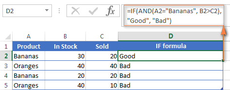
For more IF / AND formula examples, please check out his tutorial: Excel IF function with multiple AND conditions.
An Excel formula for the BETWEEN condition
If you need to create a between formula in Excel that picks all values between the given two values, a common approach is to use the IF function with AND in the logical test.
For example, you have 3 values in columns A, B and C and you want to know if a value in column A falls between B and C values. To make such a formula, all it takes is the IF function with nested AND and a couple of comparison operators:
Formula to check if X is between Y and Z, inclusive:
=IF(AND(A2>=B2,A2<=C2),"Yes", "No")
Formula to check if X is between Y and Z, not inclusive:
=IF(AND(A2>B2, A2<C2),"Yes", "No")
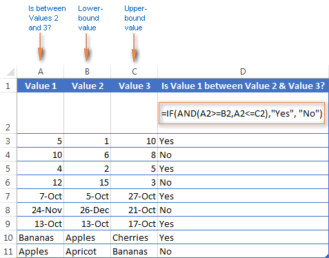
As demonstrated in the screenshot above, the formula works perfectly for all data types - numbers, dates and text values. When comparing text values, the formula checks them character-by-character in the alphabetic order. For example, it states that Apples in not between Apricot and Bananas because the second "p" in Apples comes before "r" in Apricot. Please see Using Excel comparison operators with text values for more details.
As you see, the IF /AND formula is simple, fast and almost universal. I say "almost" because it does not cover one scenario. The above formula implies that a value in column B is smaller than in column C, i.e. column B always contains the lower bound value and C - the upper bound value. This is the reason why the formula returns "No" for row 6, where A6 has 12, B6 - 15 and C6 - 3 as well as for row 8 where A8 is 24-Nov, B8 is 26-Dec and C8 is 21-Oct.
But what if you want your between formula to work correctly regardless of where the lower-bound and upper-bound values reside? In this case, use the Excel MEDIAN function that returns the median of the given numbers (i.e. the number in the middle of a set of numbers).
So, if you replace AND in the logical test of the IF function with MEDIAN, the formula will go like:
=IF(A2=MEDIAN(A2:C2),"Yes","No")
And you will get the following results:
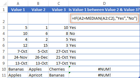
As you see, the MEDIAN function works perfectly for numbers and dates, but returns the #NUM! error for text values. Alas, no one is perfect : )
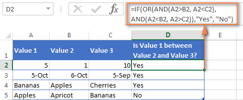
If you want a perfect Between formula that works for text values as well as for numbers and dates, then you will have to construct a more complex logical text using the AND / OR functions, like this:
=IF(OR(AND(A2>B2, A2<C2), AND(A2<B2, A2>C2)), "Yes", "No")
Using the OR function in Excel
As well as AND, the Excel OR function is a basic logical function that is used to compare two values or statements. The difference is that the OR function returns TRUE if at least one if the arguments evaluates to TRUE, and returns FALSE if all arguments are FALSE. The OR function is available in all versions of Excel 2016 - 2000.
The syntax of the Excel OR function is very similar to AND:
Where logical is something you want to test that can be either TRUE or FALSE. The first logical is required, additional conditions (up to 255 in modern Excel versions) are optional.
And now, let's write down a few formulas for you to get a feel how the OR function in Excel works.
| Formula | Description |
=OR(A2="Bananas", A2="Oranges") |
Returns TRUE if A2 contains "Bananas" or "Oranges", FALSE otherwise. |
=OR(B2>=40, C2>=20) |
Returns TRUE if B2 is greater than or equal to 40 or C2 is greater than or equal to 20, FALSE otherwise. |
=OR(B2=" ", C2="") |
Returns TRUE if either B2 or C2 is blank or both, FALSE otherwise. |

As well as Excel AND function, OR is widely used to expand the usefulness of other Excel functions that perform logical tests, e.g. the IF function. Here are just a couple of examples:
IF function with nested OR
=IF(OR(B2>30, C2>20), "Good", "Bad")
The formula returns "Good" if a number in cell B3 is greater than 30 or the number in C2 is greater than 20, "Bad" otherwise.
Excel AND / OR functions in one formula
Naturally, nothing prevents you from using both functions, AND & OR, in a single formula if your business logic requires this. There can be infinite variations of such formulas that boil down to the following basic patterns:
=AND(OR(Cond1, Cond2), Cond3)
=AND(OR(Cond1, Cond2), OR(Cond3, Cond4)
=OR(AND(Cond1, Cond2), Cond3)
=OR(AND(Cond1,Cond2), AND(Cond3,Cond4))
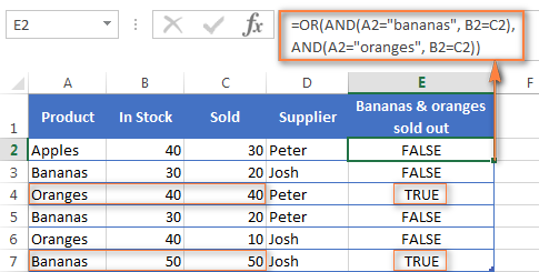
For example, if you wanted to know what consignments of bananas and oranges are sold out, i.e. "In stock" number (column B) is equal to the "Sold" number (column C), the following OR/AND formula could quickly show this to you:
=OR(AND(A2="bananas", B2=C2), AND(A2="oranges", B2=C2))
OR function in Excel conditional formatting
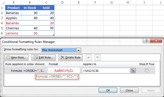
=OR($B2="", $C2="")
The rule with the above OR formula highlights rows that contain an empty cell either in column B or C, or in both.
For more information about conditional formatting formulas, please see the following articles:
Using the XOR function in Excel
In Excel 2013, Microsoft introduced the XOR function, which is a logical Exclusive OR function. This term is definitely familiar to those of you who have some knowledge of any programming language or computer science in general. For those who don't, the concept of 'Exclusive Or' may be a bit difficult to grasp at first, but hopefully the below explanation illustrated with formula examples will help.
The syntax of the XOR function is identical to OR's :
The first logical statement (Logical 1) is required, additional logical values are optional. You can test up to 254 conditions in one formula, and these can be logical values, arrays, or references that evaluate to either TRUE or FALSE.
In the simplest version, an XOR formula contains just 2 logical statements and returns:
- TRUE if either argument evaluates to TRUE.
- FALSE if both arguments are TRUE or neither is TRUE.
This might be easier to understand from the formula examples:
| Formula | Result | Description |
=XOR(1>0, 2<1) |
TRUE | Returns TRUE because the 1st argument is TRUE and the 2nd argument is FALSE. |
=XOR(1<0, 2<1) |
FALSE | Returns FALSE because both arguments are FALSE. |
=XOR(1>0, 2>1) |
FALSE | Returns FALSE because both arguments are TRUE. |
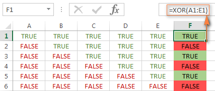
When more logical statements are added, the XOR function in Excel results in:
- TRUE if an odd number of the arguments evaluate to TRUE;
- FALSE if is the total number of TRUE statements is even, or if all statements are FALSE.
The screenshot below illustrates the point:
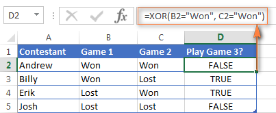
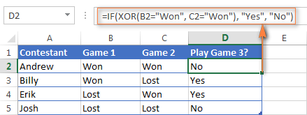
If you are not sure how the Excel XOR function can be applied to a real-life scenario, consider the following example. Suppose you have a table of contestants and their results for the first 2 games. You want to know which of the payers shall play the 3rd game based on the following conditions:
- Contestants who won Game 1 and Game 2 advance to the next round automatically and don't have to play Game 3.
- Contestants who lost both first games are knocked out and don't play Game 3 either.
- Contestants who won either Game 1 or Game 2 shall play Game 3 to determine who goes into the next round and who doesn't.
A simple XOR formula works exactly as we want:
=XOR(B2="Won", C2="Won")
And if you nest this XOR function into the logical test of the IF formula, you will get even more sensible results:
=IF(XOR(B2="Won", C2="Won"), "Yes", "No")
Using the NOT function in Excel
The NOT function is one of the simplest Excel functions in terms of syntax:
You use the NOT function in Excel to reverse a value of its argument. In other words, if logical evaluates to FALSE, the NOT function returns TRUE and vice versa. For example, both of the below formulas return FALSE:
=NOT(TRUE)
=NOT(2*2=4)
Why would one want to get such ridiculous results? In some cases, you might be more interested to know when a certain condition isn't met than when it is. For example, when reviewing a list of attire, you may want to exclude some color that does not suit you. I'm not particularly fond of black, so I go ahead with this formula:
=NOT(C2="black")
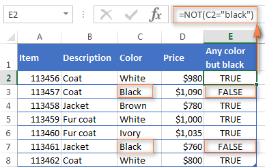
As usual, in Microsoft Excel there is more than one way to do something, and you can achieve the same result by using the Not equal to operator: =C2<>"black".
If you want to test several conditions in a single formula, you can use NOT in conjunctions with the AND or OR function. For example, if you wanted to exclude black and white colors, the formula would go like:
=NOT(OR(C2="black", C2="white"))
And if you'd rather not have a black coat, while a black jacket or a back fur coat may be considered, you should use NOT in combination with the Excel AND function:
=NOT(AND(C2="black", B2="coat"))
Another common use of the NOT function in Excel is to reverse the behavior of some other function. For instance, you can combine NOT and ISBLANK functions to create the ISNOTBLANK formula that Microsoft Excel lacks.
As you know, the formula =ISBLANK(A2) returns TRUE of if the cell A2 is blank. The NOT function can reverse this result to FALSE: =NOT(ISBLANK(A2))
And then, you can take a step further and create a nested IF statement with the NOT / ISBLANK functions for a real-life task:
=IF(NOT(ISBLANK(C2)), C2*0.15, "No bonus :(")
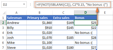
Translated into plain English, the formula tells Excel to do the following. If the cell C2 is not empty, multiply the number in C2 by 0.15, which gives the 15% bonus to each salesman who has made any extra sales. If C2 is blank, the text "No bonus :(" appears.
In essence, this is how you use the logical functions in Excel. Of course, these examples have only scratched the surface of AND, OR, XOR and NOT capabilities. Knowing the basics, you can now extend your knowledge by tackling your real tasks and writing smart elaborate formulas for your worksheets.
 by
by
564 comments
=IF("4/9/2021 12:03PM"<"4/14/2021 5:30AM",TRUE,FALSE)
The above condition gives false as output instead of true..could you please help me out
Hello!
Your dates are written as text. I recommend reading this guide: Using IF function with dates
This should solve your task.
Syntax for any of these functions requires semi-colon as separator, not comma!
=AND(($E1="valueA"); ($C1="valueB"))
Probably a question of localization settings (currency, dates etc). This is for Denmark :)
Hello Villads,
Your guess is absolutely right - the separator is determined by Regional Settings. In Denmark as well as in other European countries, List Separator is a semicolon. In North America, it's a comma. On my computer, it's also a comma :)
Hello -
Is it possible to combine IF, OR, and Match?
Ex Column A holds address values, columns B, C, D holds a VLOOKUP formula that will pull an address value from different tabs. I am trying to construct a formula that reads If A2 = B2 or A2=C2 or A2= D2 than return a value of 1 if none of these then 0. However, some of the address values are not an exact match thus returning a value of 0 (ex: A2 = 123 ABC Road and B2 = 123 ABC Rd this should = to 1 but due to Road and Rd not being the same it gives it a value of 0).
I've tried Match with a *wildcard to identify the potential match and these seems to work on its own however when I construct the entire formula it does not return the expected Value.
C58 = 123 ABC Road
J58= (Blank Value)
K58= (Blank Value)
L58 = 123 ABC Rd
=MATCH("*"&LEFT(C58,5)&"*",L58,0)
Result 1
Combined formula
IFERROR(IF(OR(MATCH("*"&LEFT(C58,5)&"*",J58,0),MATCH("*"&LEFT(C58,5)&"*",K58,0),MATCH("*"&LEFT(C58,5)&"*",L58,0)),1,0),0)
Result = 0
However anticipated result is 1
Any insight would be appreciated!
Hello!
If I got you right, the formula below will help you with your task:
=ISNUMBER(SEARCH(LEFT(C58,5),L58,1))+ ISNUMBER(SEARCH(LEFT(C58,5),K58,1))+ ISNUMBER(SEARCH(LEFT(C58,5),J58,1))
The SEARCH function finds characters in a cell.
Thank you! I was able to nest those functions into my formula and it returned the desired result 1.
=IFERROR(IF(OR(ISNUMBER(SEARCH(LEFT(C58,7),J58,1)),ISNUMBER(SEARCH(LEFT(C58,7),K58,1)),ISNUMBER(SEARCH(LEFT(C58,7),L58,1))),1,0)," ")
Hello,
Could you please help me for the below requirement.
Value 1 Value 2 Result
1 20 IF (Value1=1, Value22,Value26,Value218,Value230,4)
0 5 IF (Value1=0, Value22,Value23,Value29,Value212,4)
Hi Alexander,
I was wondering if you could help me with my formula.
=IF(OR(AND('2020-Balance Affecting'!H2>="MEMBERSHIP")*AND('2020-Balance Affecting'!H2>="RENEWAL")),'2020-Balance Affecting'!A2:M2,"FALSE")
The cell H2 on a previous tab (named "2020-Balance Affecting") in my workbook could contain more words than "membership" or "renewal" to the extent of infinite possibilities of combinations, However if either of those words are in cell H2, I would like excel to display the entire row of cells which includes the date of renewal or membership purchase and the cost involved.
Is there a way to indicate "wildcard information" containing "membership" or "renewal" in the If function's logical argument?
The function is currently selectively displaying rows no matter what text is cell H2 or outright displaying "FALSE" as desired.
examples of possibilities in cell H2 include;
2312-1065 - Renewal
1964-1066 - Renewal
Annual membership for current year. Join-now form submission
2042-1070 - Renewal
Membership Dues
etc.
My endgame is that i could pull all the membership purchases and renewals to a secondary tab in my workbook and then total the cost column. I'm not really concerned about the "FALSE" labeled rows as they would add up as a zero when I total the cost column.
Thank you for any help!
Hello!
I recommend using the FILTER function. I recommend reading this guide: Filter with multiple AND criteria.
I hope I answered your question. If something is still unclear, please feel free to ask.
Dear Sir,
Hello
i used the following formula to give me a (YES) or (NO) answer depending on the comparison LOGIC:
IF(AND($AG2>=CO$1; $AG2<CP$1);"Yes";"No"). THE FORMULA USED FOR ONE CALENDER YEAR (2015)
AG2 : IS THE DATE OF RECRUITMENT....SAY 1/1/2015 ....(m/d/y)
CO1: THE DATE of the first day of the first month of the year 2015 (1/1/2015)
CP1: THE DATE of the second month of the second month of the year (1/2/2015)
surprisingly, the formula logic is incorrect if i change the recruitment date to 25/1/2015 or even 2/1/2015. Any help will be highly appreciated
Hi, I have cells that contain variable text to display if certain conditions are met. Some of the conditions are simple, but some are a bit more complex.
Here is what I started that isn't working:
=IF(AND(New!$E$4="401(k)",OR(New!$E$4="401(k) w/ FBO","Cash Balance","Defined Benefit","Owner Only 401(k)","Owner Only 401(k) 5500-EZ","Owner Only Cash Balance"),NOT((OR("Fidelity","MassMutual","Nationwide","Not A Platform","Open Arch / Other","Securian","T Rowe Price")),Language!A7,"REVIEW"))
Basically, it is if any of these are selected (401k, 401k w/ fbo, cash balance, defined benefit, owner only 401k, owner only 401k 5500-ez, or owner only cash balance) and the one selected is not a part of Fidelity, Mass Mutual, Nationwide, Not a Platform, Open Arch/Other, Securian, or T Rowe Price, then it will display Language!A7, otherwise, we review.
Hello!
It is very difficult to understand a formula that contains unique references to your workbook worksheets.
Your explanation of the terms is not very clear.
The expression
AND(New!$E$4=”401(k)”,OR(New!$E$4=”401(k) w/ FBO”,”Cash Balance”,”Defined Benefit”,”Owner Only 401(k)”,”Owner Only 401(k) 5500-EZ”,”Owner Only Cash Balance”)
is meaningless, since it can never be executed.
I think all these conditions should be used in OR.
But your formula is not written correctly. Here's how you can write multiple OR conditions:
=IF(AND(OR(C1={"A","F","G"}),OR(D1<>{"B","C","E"})),1,0)
I hope my advice will help you solve your task.
I WANT TO KNOW WHICH FUNCTION CAN BE USED TO GET GET THE VALUE OF THE SAME IRRESPECTIVE OF WHETHER ITS PLUS OR MINUS.
EG IF A CELL SHOWS -12 OR 12 , I SHOULD GET THE ANSWER AS 12, SO I CAN USE IT IN OTHER WORKING .
Hi!
If I understand your task correctly, please have a look at this article: Absolute value in Excel: ABS function
I'm stuck and hope someone can help. =IF(H11"",TEXT(H1,"mm/dd")&"–"&TEXT(H11,"MM/DD/Y"),"") returns the correct answer but I want to add that if H11 is blank then read another cell. Possible?
Hello!
If I understand the problem correctly, replace "" in the formula with the cell address. For example:
=IF(H11 < > "",TEXT(H1,"mm/dd")&"–"&TEXT(H11,"MM/DD/Y"),G1)
I hope my advice will help you solve your task.
What if I want a formula to total how many students are new and belong to specific rep
for example it would count all item in D3-D15 that equal humberto and also E3-E15 that equal red. So the total i need has to meet both criterias from both columns
Hello!
Please check out this article to learn how to count with multiple criteria.
If something is still unclear, please feel free to ask.
I am attempting to make this calculation work any ideas:
Sorry about that. if cell G2 contains "*lab*" then divide I2/50 if not then divide I2/20. thanks
I have tried the following but have not been able to get what I need: =TRUNC(IF(ISERROR(MATCH("*lab*",G2,)),I2/50,I2/20)) as well as =TRUNC(IF(G2="*lab*",I2/50,I2/20))
Hi,
Use the following formula:
=IF(ISNUMBER(SEARCH("lab",G2,1)), I2/50 , I2/20)
You can learn more about SEARCH function in Excel in this article on our blog.
I hope this will help.
Hello,
Please advise a formula to automatically add a number for every 0.5:
Example.
0.5 - 2000
1.0 - 2500
1.5 - 3000
2.0 - 3500
Each additional 0.5 - 500
How to insert this in IF/AND statement
Regards
In D1, type 0.5 - 2000
Then in D2, type the formula
=TEXT(LEFT(D1, FIND(" - ",D1)-1)+0.5,"0.0") & " - " & TEXT(MID(D1,FIND(" - ",D1)+3,LEN(D1))+500,"0000")
Hopefully this would help you!
If any suggestions or corrections, please let me know, Alexander Trifuntov (Ablebits.com Team)
Hi
I need help
i need 6 categories
Group 1 ..................... bellow 3 months
Group 2....................... 3 to 6 months
Group 3 ....................... 6 to 9 months
Group 4.........................9 to 12 months
Group 5......................... 12 to 18 months
Group 6.......................... 18 months +
I have updated multiple If conditions but if the cell value is #N/A then it not replacing, please help some one.
=IF(D2="Red","First",IF(D2="Green","Second",IF(D2="#N/A","Third","")))
Hello!
You cannot write an error to a formula condition.
Use the formula
=IF(D2="Red","First",IF(D2="Green","Second",IF(ISERROR(D2),"Third","")))
I hope I answered your question.
Scenario:
Column A
Aug-20
Dec-20
Jan-21
Mar-21
I want Column B to populate the following:
IF A2=Dec-20 and JAN-20 then enter FY 21 in Column b2 otherwise enter FY 20
Hello!
Sorry, I do not fully understand the task.
What does the condition mean "IF A2=Dec-20 and JAN-20"? You cannot write two values in a cell.
I want to know what to do if I want to multiply a value only if it's present.
Like in a store , different type of scrolls are there and I want to multiply the scrolls value with 100 if it's present..what should be the columns and the function?
Please help someone..
Hello!
If I understand your task correctly, the following formula should work for you:
=IF(A1<>"",A1*100,"")
I hope it’ll be helpful.
I need a help ... The question is What is AND Function ?
Hi everyone!
Can you check my answer for this one? I am not sure of my answer hehe. Thank you in advance for helping me! Sorry for using your time. Stay safe and wash your hands!
Determine whether the total earning of Ms. Chan is not equal to Mr. Tan’s total earning.
Formula: =AND(H3H7)
Output: TRUE
I am not sure if I will use AND,OR ,or NOT function. Can you give me a tip when to use them? Thank you so much in advance!
its me again!
I just want to edit my comment.
it should be: =AND(H3H7)
its me again!
I can't put any symbols lol
=AND(H3H7)
if the symbols disappeared on the comment, that should be the symbol of less than and greater than. Thank you! Please help me
Hello!
I hope you have studied the recommendations in the tutorial above. It contains answers to your question.
You only have one condition. Therefore, you don't need to use AND.
=IF(H3 >= H7,TRUE,FALSE)
I hope it’ll be helpful.
Hi Sir Alexander!
Thank you for answering my question! Thank you so much for helping me and it helped a lot.
I hope you stay safe amidst this pandemic that is happening throughout the world. Stay healthy and wash your hands!
Can you help me in this one?
How: determine if the number
is zero, odd and even.
By using the MOD(to get the remainder) with IF function
Thank you in advance for helping me!!
May I suggest a simpler solution?
=NOT(H3=H7)
I need some help. Is there a function I can use to solve my problem. I have a column, that has cells that contain text with commas...below are a few examples:
Z28 = AREA, CONS, DEX
Z29 = CTM, MSC, AREA, CONS, DEX
Z30 = AREA, CONS, DEX,LHC
I am trying to solve for:
- if any cell in Z column contains any, all, or some of the following: AREA, CONS, DEX, CTM or MSC return value "Need 1"
- if any cell in Z column contains LHC return value "Need 2"
- If any cell contains LHC and any, all, or some of the following: AREA, CONS, DEX, CTM or MSC return value "Need 1 & 2"
So for example:
Z28 = AREA, CONS, DEX; value returned would be "Need 1"
Z29 = CTM, MSC, AREA, CONS, DEX; value returned would be "Need 1"
Z30 = AREA, CONS, DEX,LHC; value returned would be "Need 1 & 2"
Does this make sense?
Hello!
You can use IF and AND formula:
=IF(AND(SUM(IFERROR((FIND({"AREA","CONS","DEX","CTM","MSC"},Z28,1)),0))>0,IFERROR(FIND("LHC",Z28,1),0)>0),"Need 1&2", IF( AND(SUM(IFERROR((FIND({"AREA","CONS","DEX","CTM","MSC"},Z28,1)),0))>0,IFERROR(FIND("LHC",Z28,1),0)=0),"Need 1",
IF(AND(SUM(IFERROR((FIND({"AREA","CONS","DEX","CTM","MSC"},Z28,1)),0))=0,IFERROR(FIND("LHC",Z28,1),0)>0),"Need 2","")))
Simpler and shorter formula with CHOOSE function:
=CHOOSE(IF(SUM(IFERROR((FIND({"AREA","CONS","DEX","CTM","MSC"},Z28,1)),0))>0,1,0)+IF(IFERROR(FIND("LHC",Z28,1),0)>0,2,0),"Need 1","Need 2","Need 1&2")
I hope my advice will help you solve your task.
Hi! Need assistance...
Using AND function,
I used logical functions in two other cells and the result is TRUE for both cells. Now, I want the two cells with TRUE results as precedents for another computation with AND function. When I apply the AND referring these two cells with both True results, it give False output. Instead, the result for two referred cells with TRUE text in it, should be a true. The formula didn't prompt to an error either.. what could be the possible reason behind that....
Thanks
Hello!
Sorry, it's not quite clear what you are trying to achieve. For me to be able to help you better, please describe your task in more detail. Please specify what you were trying to find, what formula you used and what problem or error occurred. Give an example of the source data and the expected result.
It’ll help me understand it better and find a solution for you. Thank you.
Using excel formulae, find out the following
1. How many have neither registered nor completed any of the 3 courses?
2. How many have registered or trained in atleast 2 of the 3 courses?
3. How many have not been trained in any of the 3 yet?
Name SQL SAS Excel R - Registered for training (training not done yet)
Prakash R T T - Trained
Rahul R Blank - Neither
Rajiv T
Priya R T
Amit T
Karthik R
Shobha R
Prateek
Payal R
Prashant T
Anil R
Swaroop T
Tejas R
Raghav T
Sanjeev T
Madhu R
Murali
Aravind T
Balaji R
Mukundan T
Shweta R
Anusha T T
Ravi R
Rahul T
Ramya
Shriram R
Sairam T T
Srinivasan R
Trisha R
Paul T
Mani R
Venkat R
Abhishek T
Chanakya T R
Daniel R
Rishi R
Vikram R T
Prabhu R
Priya T
Mahesh R
Raj
Suresh R
Arun R
Jacob T
Malini
Mehul R
Rajeev
Sachin T R
Praphul
Diego R T
Hello!
To count the number of values for multiple conditions, use the COUNTIFS function. Please have a look at this article.
The IF function is the main logical function in Excel and is, therefore, the one to understand first. It will appear numerous times throughout this article.
For example, the ISTEXT function will check if a cell contains text and return TRUE if it does and FALSE if it does not. The NOT function is helpful because it can reverse the result of these functions.
Please assist me to correct this formula....
=IF(OR(C5:O5=0),"Open","Close")
I will update some data(it might be Alphabets, Numbers or Special Character) in respective cell from C5 to O5 and monitor the Status in P5, if any one of the cell From C5 to O5 is empty the cell P5 must return Open and if all the cell are filled then its show Closed.. Please help me to Solve this query.
Please assist me to correct this formula....
=IF(OR(C5:O5=0),"Open","Close")
Hello!
You cannot use a range in the conditions of IF, OR, AND functions. Therefore, each cell must be written separately:
=IF(OR(C5=0,D5=0,E5=0,..........),”Open”,”Close”)
Hello Alex..
Thanks for your reply..
I got it when tried with the separate cell. Again thanks for reply.
I mean a template to use for overtime calculation and task
Please i a template to use in calculating time for a task or for overtime
Can IF Function Replace XOR Function
The IF function is the main logical function in Excel and is, therefore, the one to understand first. It will appear numerous times throughout this article.
Please assist correct this formula
=,IF(H17<=$D$17*74%,"Unacceptable",IF($D$17*74%<H17<$D$17*95%,"Below Expectations",IF($D$17*95%<H17<$D$17*100%,"Competent",IF($D$17*101%<H17=$D$17*110%,"Outstanding",""))))))
Hello!
If I understand your task correctly, the following formula should work for you:
=IF(H17<=$D$17*74%,"Unacceptable", IF($D$17*74%<H17<$D$17*95%,"Below Expectations", IF($D$17*95%<H17<$D$17*100%,"Competent", IF($D$17*101%<H17=$D$17*110%,"Outstanding",""))))
Unfortunately, you did not write what data is used and what result should be obtained.
problem if Result is less or equal to 7 days than consider it 7. if result is more than 7days than cinsider actual days.
Thank you so much.
The very last one
I have a row of an approx 200 empty cells and I want to assign a number (1) at a defined interval (10.26)
The formula I'm working on is the following
IF (10.26-(C1+R1) less equal to 0.49; 1, 0)
which is working fine till I get to the cell 10
then I would like to SUM 10.26 + 10.26 so when I get to the cell 21 the next formula will be like
IF (20.52-(C21+R1) more equal to 0.49; 1, 0)
My question is: there is a way to nest the two functions and make the SUM work dinamically
maybe using a different formula altogether?
I think I was able to nest the two functions somehow
=--OR(OR(AND(10,26-(C1+R1)"less" 1*1;10,26-(C1+R1)"greater"0,49*1);
10,26-(C1+R1)"less equal"0,49*0);
OR(10,26-(C1+R1)"less equal"0,49*1;
(AND(10,26-(C1+R1)"less"1*0;10,26-(C1+R1)"greater"0,49*0))))
still I can't get around to make the sum (10.26+10.26) incremental
Hello Edoardo!
I’m sorry but your task is not entirely clear to me. Could you please describe it in more detail?
What are C1 and R1? Are these cell addresses? What cell should the first formula be in? In which cell will the second one be written, etc.?
Give an example of the expected result.
It’ll help me understand it better and find a solution for you. Thank you.
Hi Alexander,
imagine a theatre and a row of 120 seats, those are the empty cells
starting from R1,C1 to R1,C120 (row and column)
I want to assign a seat (1) every 10.26 chairs (cells)
so they are scattered irregurarly row after row.
I start counting from 1 to 10.26 and the first cell occupied (1=true) is
R1,C9 - 10.26-(1+9)= 0.26
R1,C19 - 20.52-(1+19)= 0.52
R1,C29 - 30.78-(1+29)= 0.78
To keep it irregular, each time the number is greater than 0.50
I want to move the seat to the next cell so for example R1,C19 is FALSE but R1,C20 is TRUE.
The next problem is how to make 10.26 incremental cell after cell, but probably I found a solution.
Suppose the number 10.26 is stored in the cell F4, I will use something like this
=$F$4*(COLUMN()/10-8) even if I don't know yet how it will work in multiple rows.
The first cell in my array is I2, the first row starting from I1 have the numbers from 1 to 120 (DX)
The column H store the row numbers starting with H2(0) H3(120) H4(240) and so on.
The dimension of the array is not important, it can be as little as 24 cells per row.
Thanks for your help
Hello!
I wasted a lot of time, but I don't quite understand your calculations.
I already wrote earlier - Give an example of the expected result.
Indicate which numbers should be in the first row, which numbers should be in the second row.
Then I will try to help you
last try!!
I have a row of an approx 200 empty cells and I want to assign a number (1) at a defined interval (10.26)
The formula I'm working on is the following
IF (10.26-(C1+R1)0.49; 1, 0)
My question is: there is a way to nest the two functions and make the SUM work dinamically
maybe using a different formula altogether?
is the following
IF (10.26-(C1+R1)0.49; 1, 0)
My question is:
Let's see if I can explain my problem:
I have a row of an approx 200 empty cells and I want to assign a number (1) at a defined interval (10.26). The formula I'm working on is the following
IF (10.26-(C1+R1)0.49; 1, 0)
My question is: there is a way to nest the two functions and make the SUM work dinamically maybe using a different formula altogether?
Thanks in advance for taking the time to answer my question.
Hello!
I’m sorry but your task is not entirely clear to me. Could you please describe it in more detail? Thank you!
The msg was trunkated, here it is again
Let's see if I can explain my problem:
I have a row of an approx 200 empty cells and I want to assign a number (1) at a defined interval (10.26)
The formula I'm working on is the following
IF (10.26-(C1+R1)0.49; 1, 0)
My question is: there is a way to nest the two functions and make the SUM work dinamically
maybe using a different formula altogether?
Thanks in advance for taking the time to answer my question.
how to calculate for 3 of more arguments?
below is what I mean:
Grater or equator 100 =excellent
Between 50 to 90 =very good
Less than 40 =fail
Hello!
The formula below will do the trick for you:
=IF(A1>=100,"excellent",IF(AND(A1>=50,A1<=90),"very good",IF(A1<40,"fail","")))
I hope this will help.
I have a more complicated logic function than I can work out. I am assessing building capacity and need to identify a building as 'under capacity' (where room capacity is greater than customer numbers), 'extend hours' (where room capacity is less than customer numbers, but where opening hours are equal to or less than 37.5 hours per week) and 'exceeds capacity' (where room capacity is less than customer numbers, but where opening hours are more than 37.5 hours per week OR where the room capacity is identified as 'zero').
Please help!
Hello Phil!
If I understand your task correctly, the following formula should work for you:
=IF(F1 > F2,"under capacity",IF(F3 < 37.5,"extend hours","zero"))
where
F1 - room capacity
F2 - customer numbers
F3 - opening hours
Need result as below
1. If value is > or = 0 then result will be= 80,
2. If value is <0 to -03 then result will be= 70,
3. if value is -04 to -07 then result will be= 60
4. if value is -08 to -15 then result will be= 50
-Advance thanks
Hello!
There is no need to use the AND or OR function.
The formula below will do the trick for you:
=IF(A1>=0,80,IF(A1>-3,70, IF(A1>-7,60,IF(A1>-15,50,"" ) )) )
Hi I have a similar problem to the one above but I need to make the values specific to individual suppliers
e.g IF "ACE" is the supplier but I need to specify tariffs for different pipe sizes eg <20, 20-25,40-45,50-63 etc but different suppliers have different names, size ranges and tariffs how can I write this so the correct tariff is selected for each pipe size in each supplier?
I would greatly appreciate some help with this!
Thanks in advance
Hello!
You need to search by two criteria - the name of the supplier and the size of the pipe. Perhaps this article on searching by several criteria using the INDEX + MATCH functions will be useful
I hope this will help, otherwise please do not hesitate to contact me anytime.
Fantastic, thank you very much. I will look at the article just now. I may be back for more help....
Kind regards
Leigh
Hy! Help me please with the following two tasks. Thank you very much in advance!
1. Having a personal ID number starting 1 or 5 for boys and 2 or 6 for girls, I must write in a column if that person is a girl or a boy. I tried to combine IF and XOR functions but didn`t work for me.
2. how to transform the numbers like 6,05 into text in this format: (six,05%)
Congratulations for what you are doing in helping us!
Hello!
If I got you right, the formula below will help you with your task:
=CHOOSE(--LEFT(A1,1),"Boy","Girl", "","","Boy","Girl","","","")
and
=CHOOSE(--LEFT(A6,1),"one","two","three", "four","five","six","seven", "eight","nine")& MID(A6,SEARCH(",",A6,1),10)&"%"
I hope this will help
Help. I have a working formula like this, OR(D9="X", E9="55",D9="B"), in the data validation. How can I modify this in a way that when D9="B" then only "55" value is allowed in E9? meanwhile allowing any values on E9 when D9="X"?
Thank you in advance.
Hello Miles!
If I understand your task correctly, the following formula should work for you:
OR(AND(E9="55",D9="B"),D9="X")
I hope it’ll be helpful.
I want in excel sheet, 5+6+7*+8= 26. (*) it's cricket talk Batsman Not Out.
How I put in excel sheet.
Hello Sanjoy!
I’m sorry but your task is not entirely clear to me. Could you please describe it in more detail? What is "cricket talk Batsman Not Out"?? Also write what exactly you want to receive.I will try to help you.
CURR. T. INV. VALUE VALUE CONVERTED IN AED
USD 11,545.00 (CURRENCY(1)=VALUE IN AED) * INV VALUE = TOTAL CONVERSION VALUE
EUR 1,199.00
KWD 2,000.00
AED 5,000.00
QAT 12,000.00
GBP 1,500.00
USD 3.674
EUR 3.99
KWD 11.9
AED 1
QAT 1.01
GBP 4.59
Can anyone help me with the formula for the above.
If I enter the currency whether it's Eur or USD the amount will be converted automatically and whatever the conversion is, it will be multiplied by Column 2 (Total Value) and the total conversion will be on column 3.
Appreciate you help.
Hello Jane!
To show the rate for a necessary currency in cell C2, you can use this formula:
=VLOOKUP(A2,$A$10:$B$15,2,0)
$A$10:$B$15 is your table with the currency rate, A2 is a cell where the currency is specified (USD in your case).
Please read more about the VLOOKUP function here.
If you have any additional questions, I will be happy to answer them.
=IF(AND(E3<6,OR(TIME(11,45,0)<F3<TIME(12,0,0),TIME(18,45,0)<F3<TIME(19,30,0))),"early bird", "")
write a logical function to find out whether a customer is an early bird. (refer to the 'Early Bird' criteria stated above) In your function, you will have to reference Column E values (day of week) and Column F (time of order) to determine whether customers are early birds. Think about how you will reference the early bird criteria.
E3= weekday number (1-7)
f3 time 7:12pm
Early Bird criteria - Customers who want to avail of an Early Bird discount must place their orders on weekdays between 11:45 a.m. - 12:00 p.m. (for lunch) or 6:45 p.m. - 7:30 p.m. (for dinner).
can somebody help,
Hello Neha!
If I understand your task correctly, the following formulas should work for you:
=IF(AND(E3 < 6,OR(AND(TIME(11,45,0) < F3, F3 < TIME(12,0,0)), AND(TIME(18,45,0) < F3,F3 < TIME(19,30,0)))), "early bird", "")
Hope you’ll find this information helpful.
thanks this note are very helpful to me as a student
Does RIGHT,LEN,FALSE belong to the logical category
Hi!
FALSE is categorized under Logical functions; RIGHT and LEN belong to the category of Text functions.
I need help please, i need to a formula about this problem, from jan. 26,2019 to feb. 25, 2019 there are four fridays and 27 working days. The thing i need is on calculating working days minus the working hours for the whole month, see below example
BG5 BH5 BI5
Total Working Hrs Total Regular Hrs Total Overtime Hrs
is from jan26 to feb25 is only 260 hrs is what i also need formula
and the january month has 31 therefore the total days until february 25 is also 31 days but i need only 26 working days and 4 days fridays. I tried the formula for total overtime as this:=IF(BG5=>BH5,BG5-BH5,0) it only applies when there is only 30 days a month and 4 fridays but does not gave me when there are 5 fridays in a month and also if there is 31th day of the month.
Any help is Greatly appreciated!
If cell B2 = 43830 (which is December 31, 2019 and assuming that cell B2 does say December 31, 2019) and if (-5 + 2 +7)>0 which is also true, how do I write this to make it work in an IF/AND statement?
Any help is Greatly appreciated!
=if(and(b2=date(2019,12,31),(-5+2+7)>0),"value if true","value if false")
This article was extremely well-made and useful. Thanks! One question tho, when using a formula with the same format as =OR($C1"", $D2"") , could I instead do =OR(C1:C2"") ?
Hi all,
I need assistance with the following conditions for a sales model.
The user wants to sell widgets and they do not want be charged for the 1st 5000 sales. They will then be billed $20 for each widget over 5000 sales. They also only want to pay for a maximum number of widgets (10,000) even if sales exceed this level.
Any assistance would be greatly appreciated.