This blog post covers those Google Sheets functions that Excel doesn't offer. They are conveniently classified by their primary task. Whether you're managing data, translating text, or visualizing information, these Google Sheets functions are invaluable additions to your toolkit.
Exclusive Google Sheets functions
The first group includes those Google Sheets functions that fall under the Google category. They offer unique capabilities for specific cases.
Google Sheets ARRAYFORMULA
Typically, Google Sheets formulas work with one cell at a time. However, scanning and calculating entire ranges of cells will significantly save you time. This is where Google Sheets array formulas come to play.
Array formulas are like more powerful versions of regular formulas. They process entire ranges of cells — as many rows or columns as your formula contains. Besides, they make non-array formulas work with arrays, too!
In Excel, you have to remember to finish a formula with Ctrl+Shift+Enter to turn it into an array formula. The curly brackets at both ends of the formula will indicate success.
In Google Sheets, this is simplified with a special function:
You put your entire Google Sheets formula with ranges inside the standard round brackets and finish as usual — by hitting Enter.
The simplest example would be with the IF function for Google Sheets.
Suppose you have a table with survey results on Sheet1. The table is linked to a form so it is updated constantly. Column A contains respondents' names and column B contains their answers — yes or no.
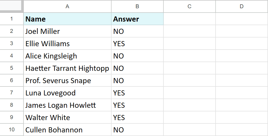
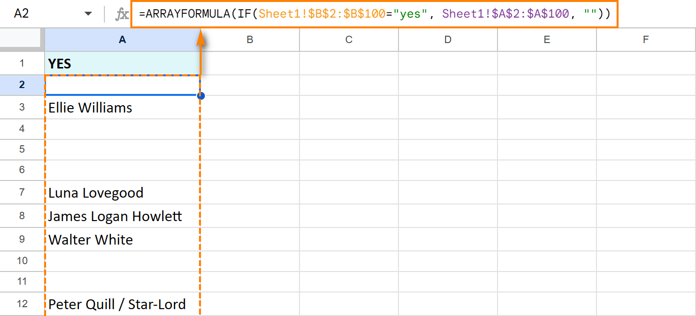
You need to display the names of those who said yes on Sheet2.
While IF usually refers to one cell, Google Sheets ARRAYFORMULA lets your IF process all names and responses at once. Here's the formula to use on Sheet2:
=ARRAYFORMULA(IF(Sheet1!$B$2:$B$100="yes", Sheet1!$A$2:$A$100, ""))
GOOGLEFINANCE function
Have you ever wondered if it's possible to track currency exchange rates in Google Sheets? Or find out the cost of an item in your country's currency? And maybe even how much did it cost a week ago? A month or a year ago?
Google Sheets answers all these and some more questions with the GOOGLEFINANCE function. It connects to Google Finance servers and fetches current or historical financial information right into your spreadsheet.
Let me briefly explain each GOOGLEFINANCE argument:
- Though the function contains quite many arguments, only the first one — ticker — is truly required. is truly required. Google Sheets function will consider the ticker symbol here to fetch the info. For example, GOOG stands for Google, MSFT — for Microsoft.
Other arguments are optional and their usage depends on what you're trying to get:
- attribute is whatever you're looking for. If omitted, it is "price" by default. But if you need the info on a certain day, you need to enter this part of the formula anyway. You can also fetch the current day's high price ("high"), the previous day's closing price ("closeyest"), or the price as of when the market opens ("priceopen").
Tip. You will find the full list of attributes in this Google Docs Editors Help for GoogleFinance.
- start_date and end date|num_days are used to specify the period over which you want to check the data. You enter the first day of the period, and either the last day or the number of days after the first date.
- interval tells the frequency at which to return the data. It can either be "daily" (1) or "weekly" (7).
Here are several simple examples of how you use the GoogleFinance function.
Example 1. Current stock price
Fetch the current stock price of Google, Microsoft, Nvidia and Netflix from the American stock exchange called Nasdaq:
=GOOGLEFINANCE("NASDAQ:GOOG", "price")

Example 2. Historical stock price
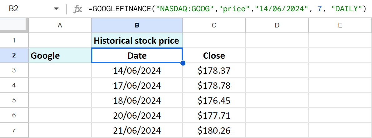
Similarly, you can retrieve the stock prices for the last 7 days:
=GOOGLEFINANCE("NASDAQ:GOOG","price","14/06/2024", 7, "DAILY")
Example 3. Current exchange rate
GOOGLEFINANCE also helps to fetch currency exchange rates:
=GOOGLEFINANCE("CURRENCY:EURGBP")
to get rates for turning euros into pound sterlings=GOOGLEFINANCE("CURRENCY:GBPUSD")
to fetch the info on converting pound sterlings to US dollars=GOOGLEFINANCE("CURRENCY:USDEUR")
how much does switching from US dollars to euros cost

Example 4. Historical exchange rate
Or check the exchange rates from the same day a year ago:
=GOOGLEFINANCE("CURRENCY:EURGBP","price","25/06/2023")
=GOOGLEFINANCE("CURRENCY:GBPUSD","price","25/06/2023")
=GOOGLEFINANCE("CURRENCY:USDEUR","price","25/06/2023")

Google Sheets function to detect language
Have you ever received data with text in multiple languages and needed to identify the language of each piece of text? Google Sheets has a unique function for that — DETECTLANGUAGE.
It scans the provided text and returns the detected language code. This function can be incredibly useful when dealing with multilingual datasets (for localization, etc.)
Suppose you have text in column A. Use the DETECTLANGUAGE function in column B to identify the language of each text string:
=DETECTLANGUAGE(A2)
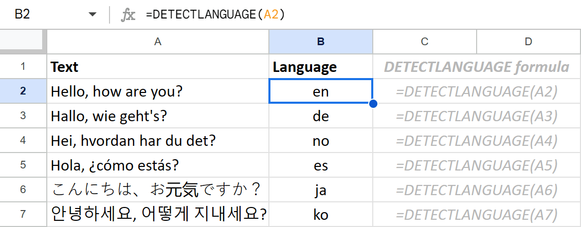
It will return the language codes (e.g., "en" for English, "no" for Norwegian) for each cell in column A.
Google Sheets function to translate language
Need to translate text directly in your spreadsheet? Google Sheets offers the GOOGLETRANSLATE function, which uses Google Translate to convert text from one language to another.
- specify the text (cell with the text) you want to translate
- provide the code of the source_language (use "auto" for Google Sheets to detect the language automatically)
- provide the code of the target_language (omit to translate to your system language)
For example, make Google Sheets formula to detect the language in column A and translate each phrase to English:
=GOOGLETRANSLATE(A2,"auto","en")

Google Sheets QUERY function
I believe QUERY in Google Sheets is the most comprehensive and powerful function you can find. It is used in so many different ways that I can't list them all.
It can fully substitute the Google Sheets FILTER function, it can sort your data, count, sum, and apply the AVERAGE function.
All in all, formulas built with Google Sheets QUERY let you handle large datasets easily. It uses a special Query Language — a set of commands that regulate what the function does.
Tip. If you're familiar with databases, these commands may remind you of SQL.
Tip. Don't want to figure out any commands? I hear you ;) Hop below to learn about the tool that will build Google Sheets QUERY formulas for you.
I won't explain every detail here because I did it in this separate article. But to stir up your interest, I'll show you a few examples.
How do you pull data by date and/or by text (by condition)?
A special clause where lets you specify the condition that should be met to return specific rows only. This endows Google Sheets QUERY with filtering powers.
- Get the list of those movies that aired after the '60s:
=QUERY(Movies!A1:C10, "select A,C where C > 1960")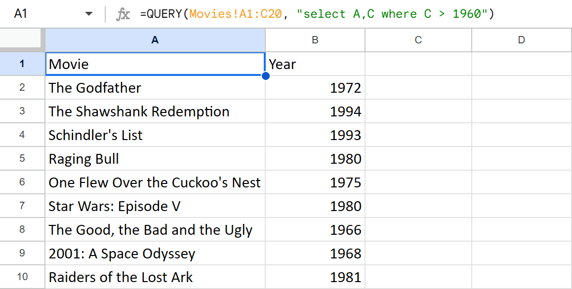
- Or pick all dramas that aired after 1950 only (those movies where Drama appears in the Genre column):
=QUERY(Movies!A1:C20,"SELECT * WHERE (lower(B) contains 'drama') AND (C > 1950)")
Generate QUERY formulas automatically
Formulas are great and all, but if you have neither time nor desire to learn them, the following add-on will help you immensely.
Filter and Extract Data creates QUERY formulas for you without needing to understand the full syntax of the QUERY language.
Using this add-on, you will:
- Pull various columns from another sheet based on multiple criteria.
- Filter data using simple drop-down lists.
- Preview the resulting QUERY formula and the data it will return.
And all of these in just one intuitive window:
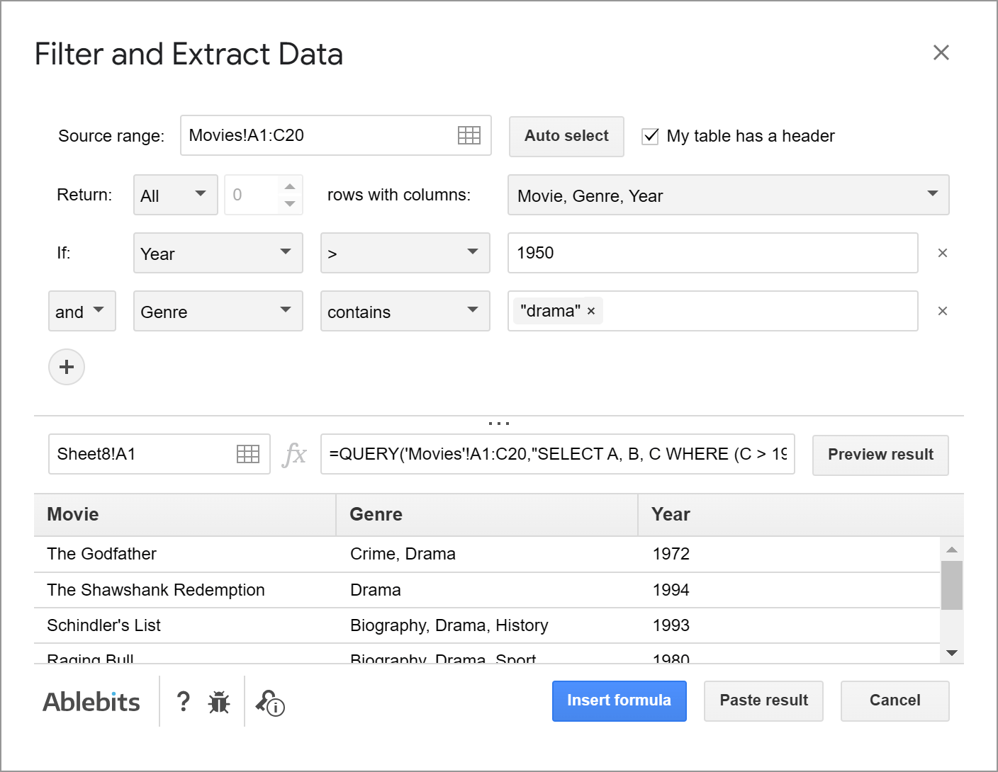
If you don't need QUERY formula and rather have its result, get only values pasted to your sheet by hitting Paste result button instead of Insert formula at the bottom.
Install Filter and Extract Data to your spreadsheets from the Google Workspace Marketplace to work with complex data queries easily without the need to manually wrote formulas.
Visit the add-on help page to see all options it has to offer or watch this 5-min demo-video:
See what else QUERY can do:
Google Sheets SPARKLINE function
Creating quick, in-cell charts has never been easier than with the SPARKLINE function in Google Sheets. Unlike traditional chart tools, SPARKLINE is a lightweight function that generates simple, compact charts within a single cell.
- select the range with data for the chart
- set up extra options for the chart such as type, axis length, colors. (If you don't mention anything, the function will return a black line chart by default.)
I have a short list of incomes over the year. Let's try and build small charts based on that data.
Example 1. Line chart
I merge 6 cells for the chart to look good and enter the following formula there:
=SPARKLINE(B2:B10)
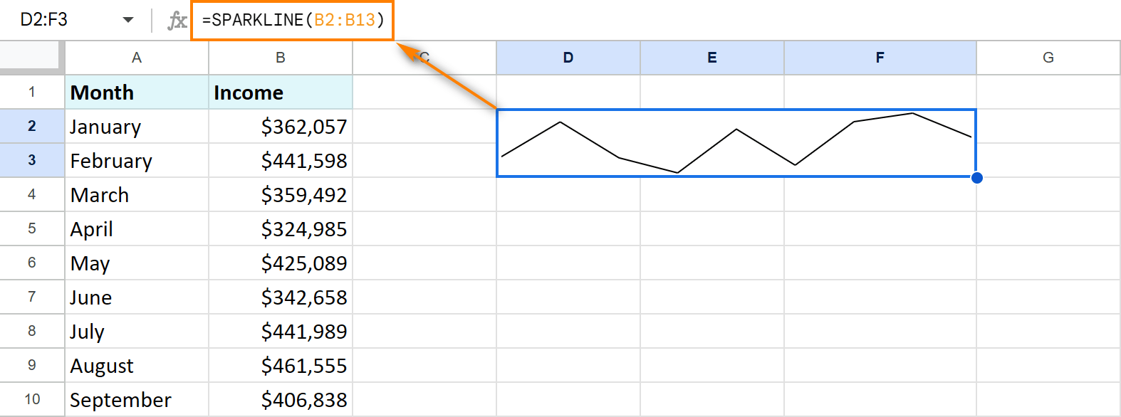
You will see a line chart like this as a default one if you don't specify anything but the range of cells.
Example 2. Column chart
To change the type of the chart, I will need to use the first option — charttype — followed by the type of the chart itself — column.
Note. Each command should be wrapped in double-quotes while the entire pair put to curly brackets.
=SPARKLINE(B2:B10, {"charttype", "column"})
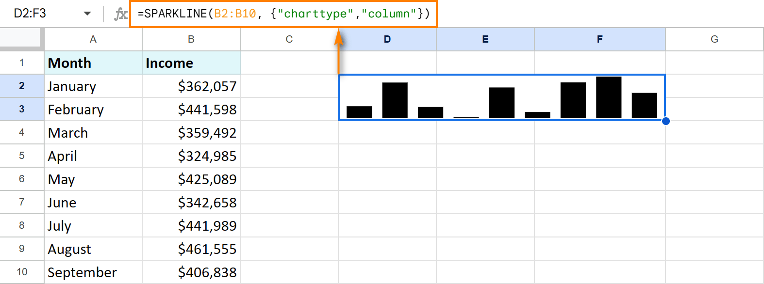
Example 3. Fine-tune the chart
The next thing I'm going to do is specify colour.
Note. Each new pair of clauses should be separated from the previous one by a semicolon.
=SPARKLINE(B2:B10, {"charttype", "column"; "color", "orange"})
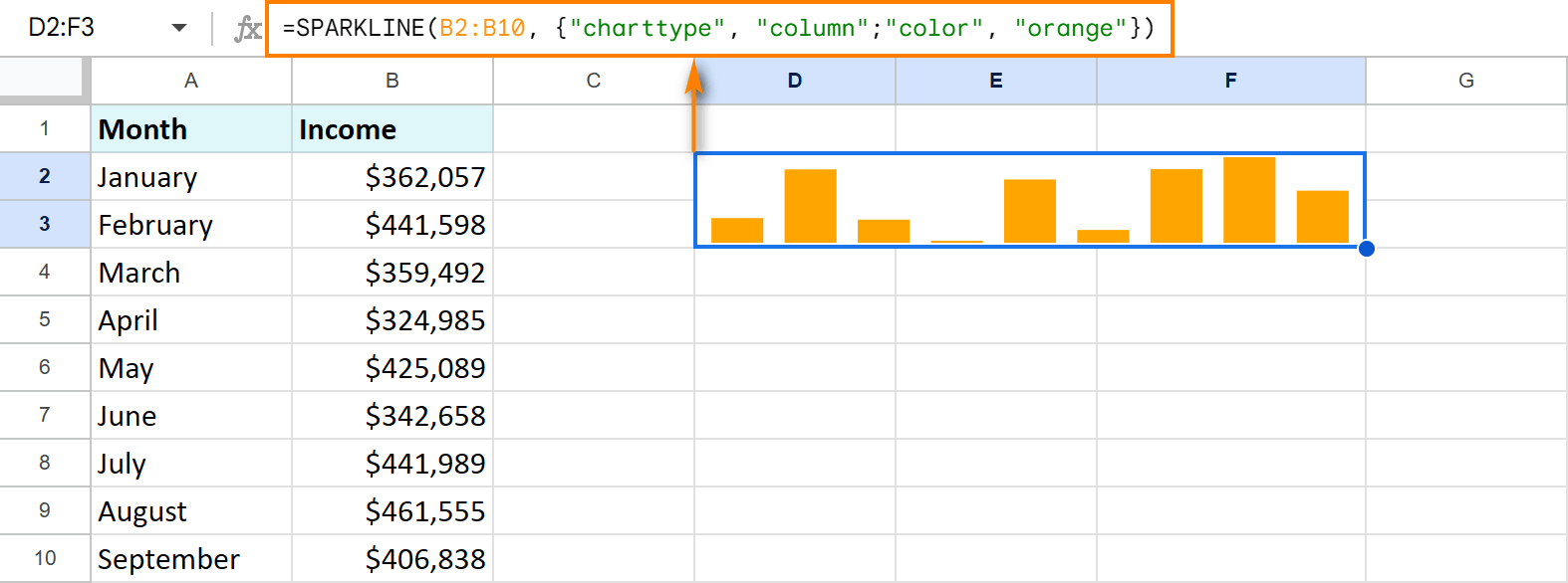
Google Sheets SPARKLINE lets you set different hues for the lowest and highest records, specify how to treat blanks, etc.
Tip. You will find a full list of commands in this tutorial.
Google Sheets function to sort and filter — SORTN
Google Sheets takes sorting to the next level with the SORTN function. While the SORT function allows basic sorting, SORTN adds the ability to return only the top n rows, based on specified criteria.
For example, how do you return the top 5 rows from columns A and B while sorting them by column B in descending order? With this formula:
=SORTN(A2:B10, 5, 0, 2, TRUE)
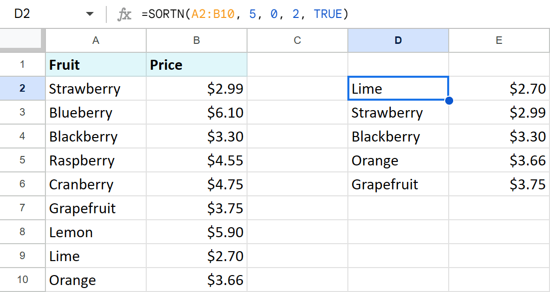
Tip. You can read more about Google Sheets SORTN on its Docs Editor Help page.
Google Sheets math function — COUNTUNIQUE
Ever wondered how to count unique records in spreadsheets instead of pulling them to a separate list? Well, here's a Google Sheets function for you that does that:
You can list as many values, cell references or ranges as you need right in the formula.
Note. Unlike UNIQUE, the function cannot count entire rows. It deals with individual cells only. Thus, each new cell in another column will be treated as unique.
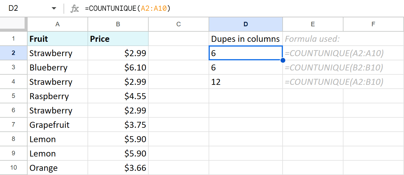
Formula examples:
- count unique entries in column A:
=COUNTUNIQUE(A2:A10) - count unique entries in column B:
=COUNTUNIQUE(B2:B10) - count unique entries in both columns A and B:
=COUNTUNIQUE(A2:B10)
See also:
Import data from the Web
Were it not for certain Google Sheets functions, importing data from other spreadsheets and the Web would be a pain in the neck.
How to use IMPORTRANGE in Google Sheets
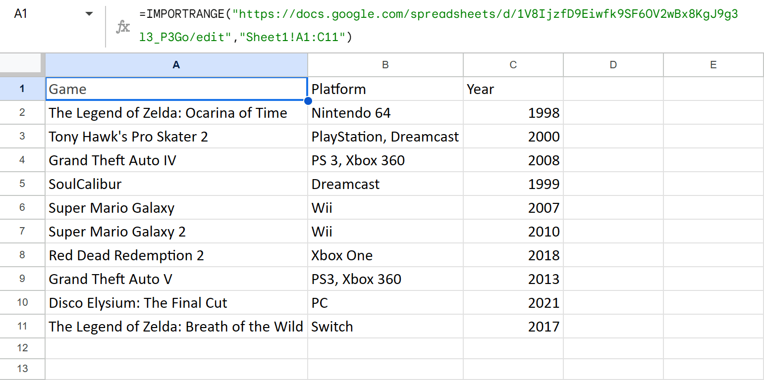
The IMPORTRANGE function lets you pull data from other documents in Google Sheets:
You just specify a spreadsheet_url of the file with your source sheet, and enter the range_string that you want to import.
=IMPORTRANGE("https://docs.google.com/spreadsheets/d/1V8IjzfD9Eiwfk9SF6OV2wBx8KgJ9g3l3_P3Go/edit","Sheet1!A1:C11")
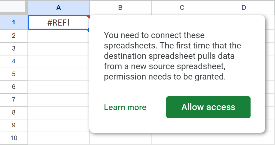
Note. The first time you reference another file, the formula will return the error. No need to panic. The thing is, before IMPORTRANGE for Google Sheets can fetch the data, you will have to permit it to access another spreadsheet. Just hover your mouse over that error and you'll see Allow access button that will help you do that:
Tip. I discussed IMPORTRANGE in detail in one of the previous blog posts, have a look.
IMPORTHTML and IMPORTDATA
These two Google Sheets functions are designed to import data from web pages and online sources into spreadsheets without manual copy-pasting.
-
IMPORTHTML(url, query, index)
Use this Google Sheets function to import data from tables or lists on web pages.
- provide the URL of the web page
- decide if you want to get a "list" or a "table"
- and if there are several tables or lists on the page, specify which one you need by supplying its number
=IMPORTHTML("https://travel.gc.ca/travelling/advisories", "table", 1)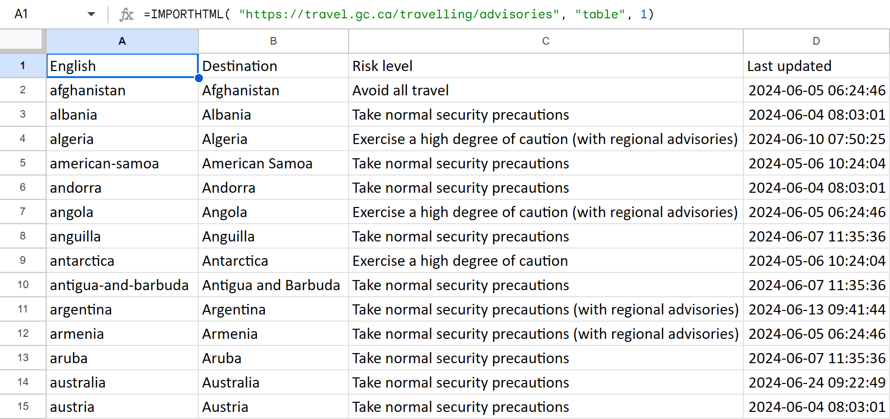
-
=IMPORTDATA(url)
Just provide the URL of your source page or a reference to a cell with such a link.
Google Sheets functions to convert numbers
Google Sheets offers a few specialized functions to convert numbers into different formats:
- TO_DATE
Converts a serial number to a date. It's equivalent to applying Format > Number > Date time from the spreadsheet menu.
=TO_DATE(43882)This converts the serial number 43882 to the corresponding date.
- =TO_PERCENT
Converts a decimal number to a percentage. It's equivalent to applying Format > Number > Percent from the spreadsheet menu.
=TO_PERCENT(0.85)This converts 0.85 to 85%.

…Phew! What a crowd of exclusive Google Sheets functions! :) Can you believe Excel doesn't have these? I bet they take Google Sheets to the next level in data processing.
If you come across any other Google Sheets functions that Excel lacks, or if you have any tips and tricks to share, I'd love to hear from you in the comments section below!
 by
by 
14 comments
How do you reference a cell in the same spreadsheet and write to it. For example I am in C2 and would want to write something to D2 based on the data in C2.
Hello Pav,
If I understand you correctly, entering =C2 into D2 will do the trick. Feel free to read this article to learn other basic operations: Create and edit Google Sheets formulas
Hi, I need to combine 4 sheets that contains around 100 tabs each. It would be hard to name all tabs in an IMPORTRANGE Function.
Is there a way to do it with a QUERY function? I have programming background but I don’t know where to start.
Can you please advise? Thank you very much
Hi Alicia,
To combine data from different files, you will still need to use the IMPORTRANGE function. It's the only way to transfer data between different spreadsheets in Google Sheets.
However, there's a Combine Sheets add-on that will help you do that quickly. It is described in this blog post along with other possible ways, feel free to take a look.
Does SUMIFS work from IMPORTRANGE? I tried to use SUMIFS from a range imported from a different google sheet, and I received "0". There was no other syntax error.
Hello Nik,
I'm afraid you will have to import the range with a standalone function first and then apply SUMIFS.
Alternatively, you can use the QUERY+IMPORTRANGE combo since QUERY knows how to sum by your criteria as well.
Thank you so very much! I love reading your articles and I learn alot.?☺?☺?
Appreciate your kind words, Aekaterini! It's good to know our articles help :)
Interesting. Although there is now a filter and sort option in excel 365. Used with unique, it's quite powerful
Hi Andrew,
That's the beauty of Google Sheets where these functions are available to everyone :)
Hi!
I want to use IMPORTRANGE to merge several google sheets (those sheets are provided with format and with the same template), however what I want to see or import only are certain rows with data on it, not the whole template per sheet.
Say I have 5000 rows on each sheets, File 1 has 500 rows with data, File 2, has 200, & File 3 has 100 rows have data only, how can I apply IMPORTRANGE on this scenario since as per example there are no added condition after the string_range
Hoping for your positive response.
Hi Jess,
You can limit the number of rows to return manually in the second argument of the IMPORTRANGE.
But if you want the formula to do that automatically, try wrapping IMPORTRANGE in the QUERY function. You'll be able to make QUERY check and pull all non-empty rows using IMPORTRANGE. You'll find more details in the following blog post: Google Sheets QUERY to import ranges
Hi there!
I need to get the stock price at the specific time.
I use this formula : =GOOGLEFINANCE("NASDAQ:GOOG"; "price";time(15;55;0)) but the result still error
At this example I want to get the stock price at 5 minutes before closing.
is it possible?
give me an advice on how to solve this matter. Thanks
Hello!
The GOOGLEFINANCE function can show data for a certain date only at the beginning or at the end of a trade. Data cannot be shown at any other point in time. You can see more detailed information here.