Today's blog post features all ways to merge Google Sheets: as many as you need. You will learn to use VLOOKUP, INDEX/MATCH, QUERY and Merge Sheets add-on. All of them update cells in one sheet from records from other ones based on matches in common columns.
1. Merge Google sheets using VLOOKUP function
The first thing you may turn to when you need to match and merge Google sheets is the VLOOKUP function.
VLOOKUP syntax & usage
This function scans a column you specify for a certain key value. Once the match is there, it pulls the related records from the same row into another table or sheet.
Though Google Sheets VLOOKUP is usually considered one of the difficult functions, it's super straightforward once you get to know it.
Let's take a quick look at VLOOKUP components:
- search_key is the key value you're looking for. It can be any text string, number, or a cell reference.
- range is that group of cells (or a table) where you will look for the search_key and where you will pull the related records from.
Note. VLOOKUP in Google Sheets always scans the first column of the range for the search_key.
- index is the number of the column within that range where you want to pull the data from.
E.g., if your range to search is A2:E20 and it's column E you need to get the data from, enter 5. But if your range is D2:E20, you'll need to enter 2 to get records from column E.
- [is_sorted] is the only argument that you can omit. It's used to say if the column with key values is sorted (TRUE) or not (FALSE). If TRUE, the function will work with the closest match, if FALSE — with a complete one. When omitted, TRUE is used by default.
Tip. We have a detailed guide on VLOOKUP in Google Sheets. Please check it out to learn more about the function, its peculiarities & limits, and get more formula examples.
With these arguments in mind, let's use VLOOKUP to merge two Google sheets.
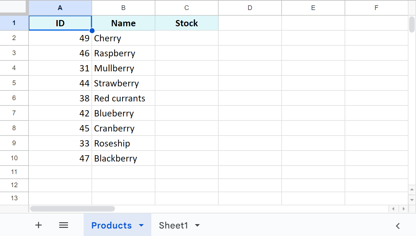
I have my main table with berries and their IDs in the Products sheet. Stock availability is unknown though:
There's also another table in Sheet1 with all data in place, including stock availability:
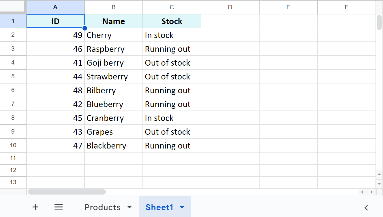
It'll be my lookup table since I will look into it to get the data.
I will use Google Sheets VLOOKUP to merge these sheets:
- It will first match berries in both tables.
- And then pull the corresponding "stock" info from the lookup into the main table.
=VLOOKUP(B2,Sheet1!$B$2:$C$10,2,FALSE)
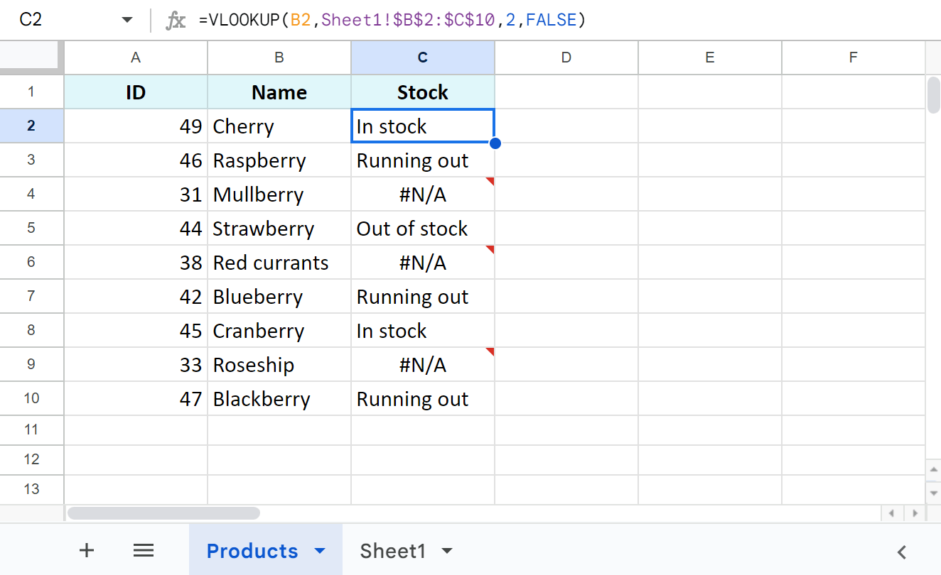
Here's how this VLOOKUP merges Google sheets exactly:
- It looks for the value from B2 (main sheet) in column B on Sheet1 (lookup sheet).
Note. Remember, VLOOKUP scans the 1st column of the specified range — Sheet1!$B$2:$C$10.
Note. I use absolute references for the range because I copy the formula down the column. This way, this range will stay the same in every row and the result won't break.
- FALSE at the end says that data in column B (in the lookup sheet) is not sorted so only exact matches will be considered.
- Once there's a match, Google Sheets VLOOKUP pulls the related record from the 2nd column of that range (column C).
Catch VLOOKUP errors in Google Sheets — IFERROR
But what about those #N/A errors?
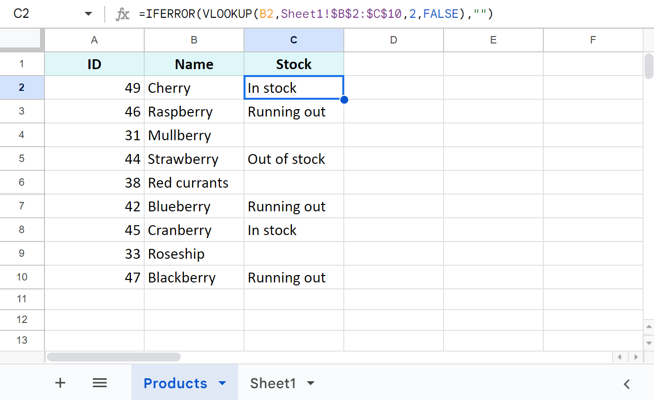
You see them in those rows where berries don't have matches in another sheet and there's nothing to return. Luckily, there's a way to keep such cells empty instead.
Just wrap your Google Sheets VLOOKUP in IFERROR:
=IFERROR(VLOOKUP(B2,Sheet1!$B$2:$C$10,2,FALSE),"")
Tip. If your Google Sheets VLOOKUP returns some other errors, you will trap and fix them using solutions from this guide.
Match & update entire column at once — ArrayFormula
One more trick I have to share is how to match and merge Google Sheets for the whole column at once. Nothing fancy here, just one more function — ArrayFormula:
- Simply replace your one-cell reference (B2) in Google Sheets VLOOKUP with the entire column (B2:B10).
- And put this whole formula inside the ArrayFormula function.
=ArrayFormula(IFERROR(VLOOKUP(B2:B10,Sheet1!$B$2:$C$10,2,FALSE),""))
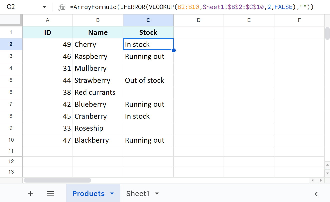
This way, you won't need to copy your VLOOKUP down the column. ArrayFormula will pull the correct result for each cell right away.
Tip. Find more details about ArrayFormula in this blog post.
Although VLOOKUP in Google Sheets is perfect for such simple tasks, it has a major drawback: it can't look at its left. Whatever range you indicate, it always scans its first column.
Thus, if you need to merge two or more Google sheets, and for example pull IDs (1st-column data) based on berries (2nd column), VLOOKUP won't help.
In cases like this, INDEX MATCH for Google Sheets enters the game.
2. Match & merge Google sheets using INDEX MATCH duo
INDEX MATCH, or rather INDEX & MATCH, are actually two different Google Sheets functions. But when they are used together, it's like a next-level VLOOKUP.
Yes, they also merge Google sheets: update cells in one table with records from another table based on matching key records. But they ignore all those limitations VLOOKUP has doing a much better job!
I won't cover all the basics below because I did that in this blog post. But I will show you how to use INDEX MATCH to specifically merge Google sheets. I will use the same sample tables from above.
1. Update data to the right of the matching column
First, let's merge those Google sheets and update the stock availability for all matching berries:
=INDEX(Sheet1!$C$1:$C$10,MATCH(B2,Sheet1!$B$1:$B$10,0))
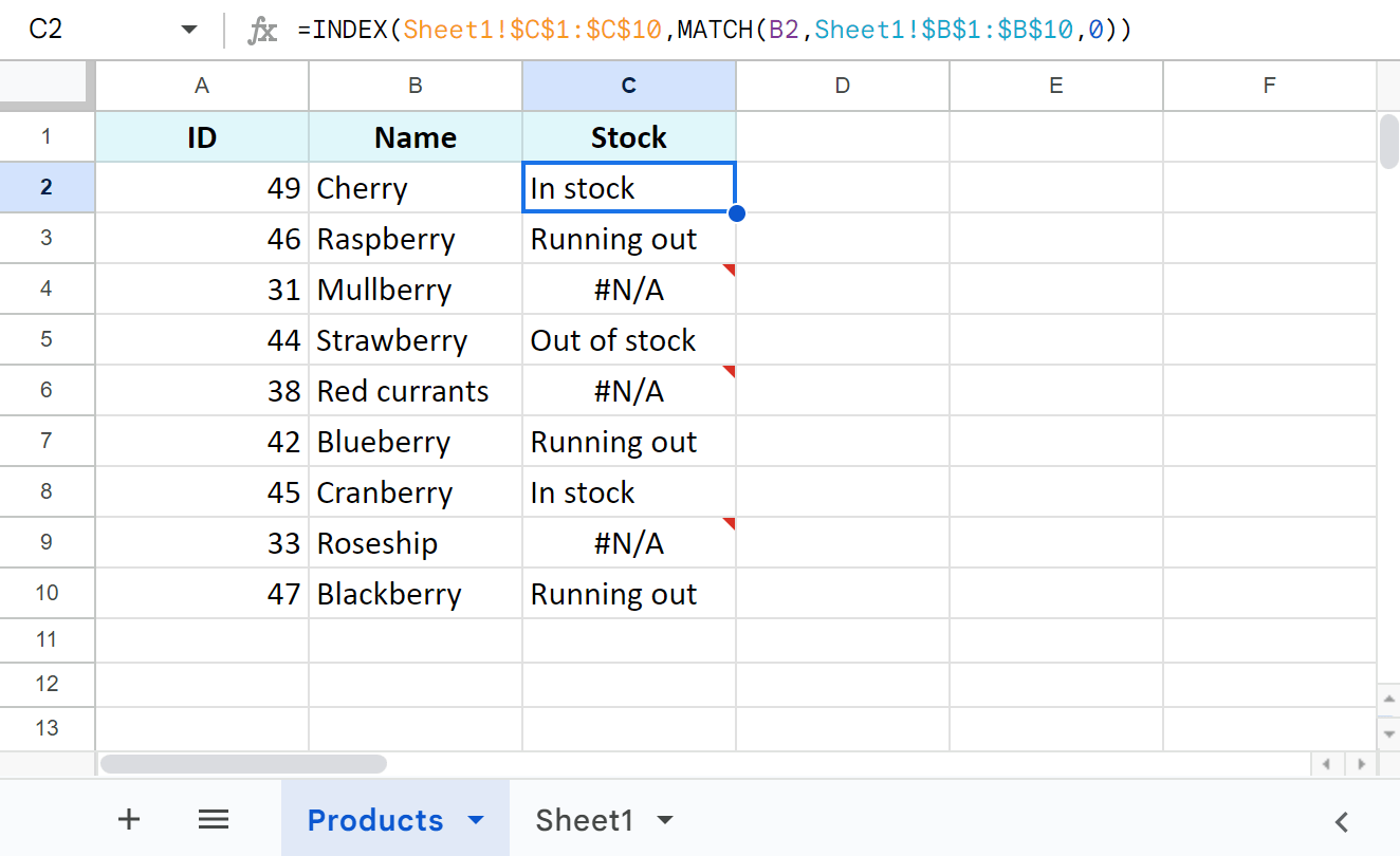
How do INDEX & MATCH merge sheets like that?
- MATCH looks at B2 and searches for the exact same record in column B on Sheet1.
- Once found, it returns the number of the row that contains that value — 10 in my case.
- INDEX goes to that 10th row on Sheet1 as well, only it pulls the value from another column — C.
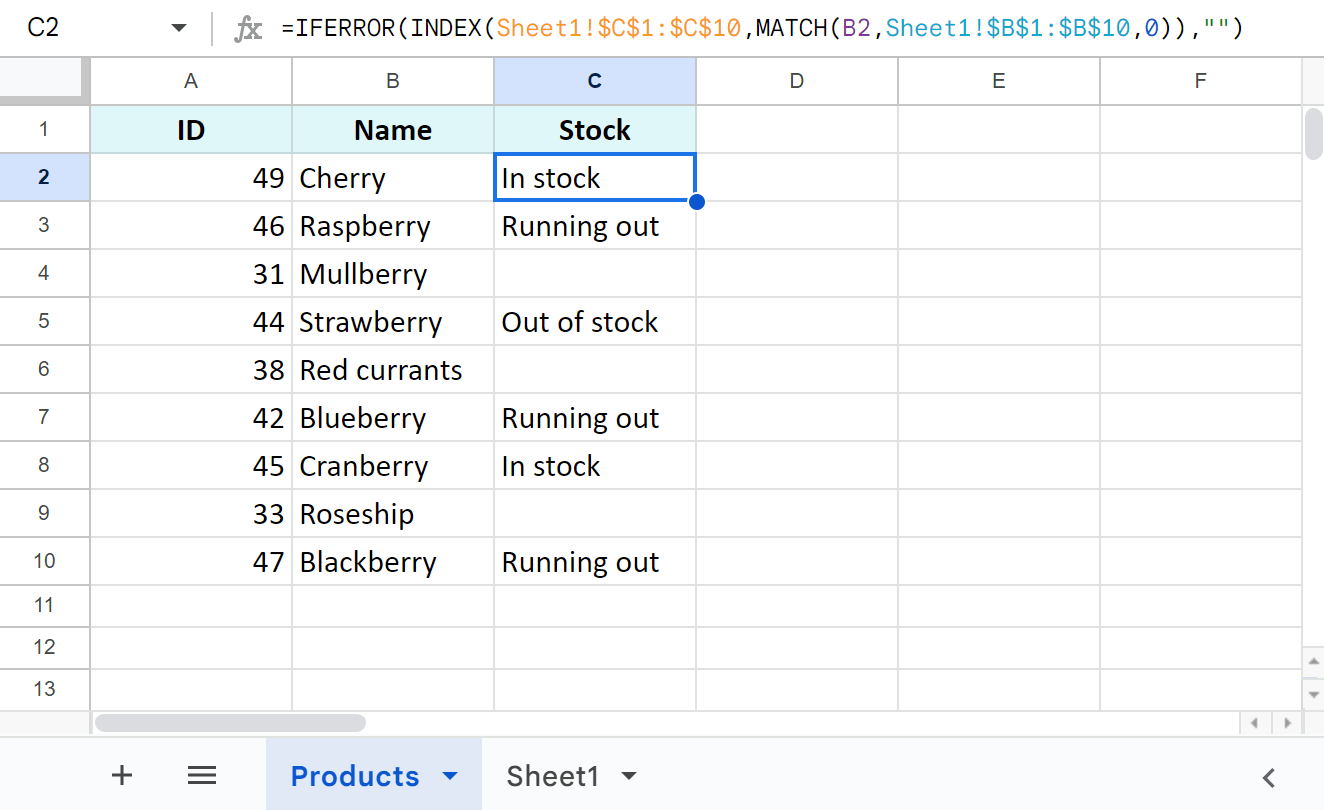
One common thing INDEX MATCH have with VLOOKUP is errors in cells with no matches. The solution is also the same: IFERROR will help again. Just put your Google Sheets INDEX MATCH as its first argument.
=IFERROR(INDEX(Sheet1!$C$1:$C$10,MATCH(B2,Sheet1!$B$1:$B$10,0)),"")
2. Update data to the left of the matching column
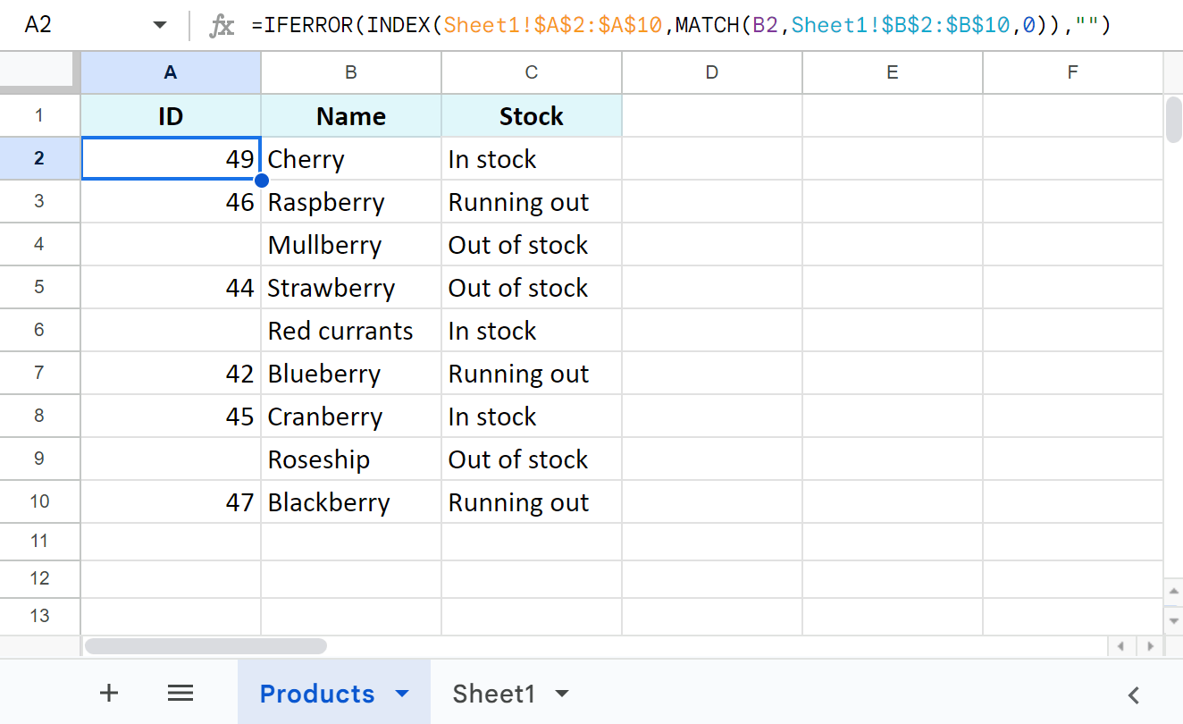
Now let's try and test INDEX MATCH against what VLOOKUP cannot do — merge Google sheets and update the leftmost column with the required IDs:
=INDEX(Sheet1!$A$2:$A$10,MATCH(B2,Sheet1!$B$2:$B$10,0))
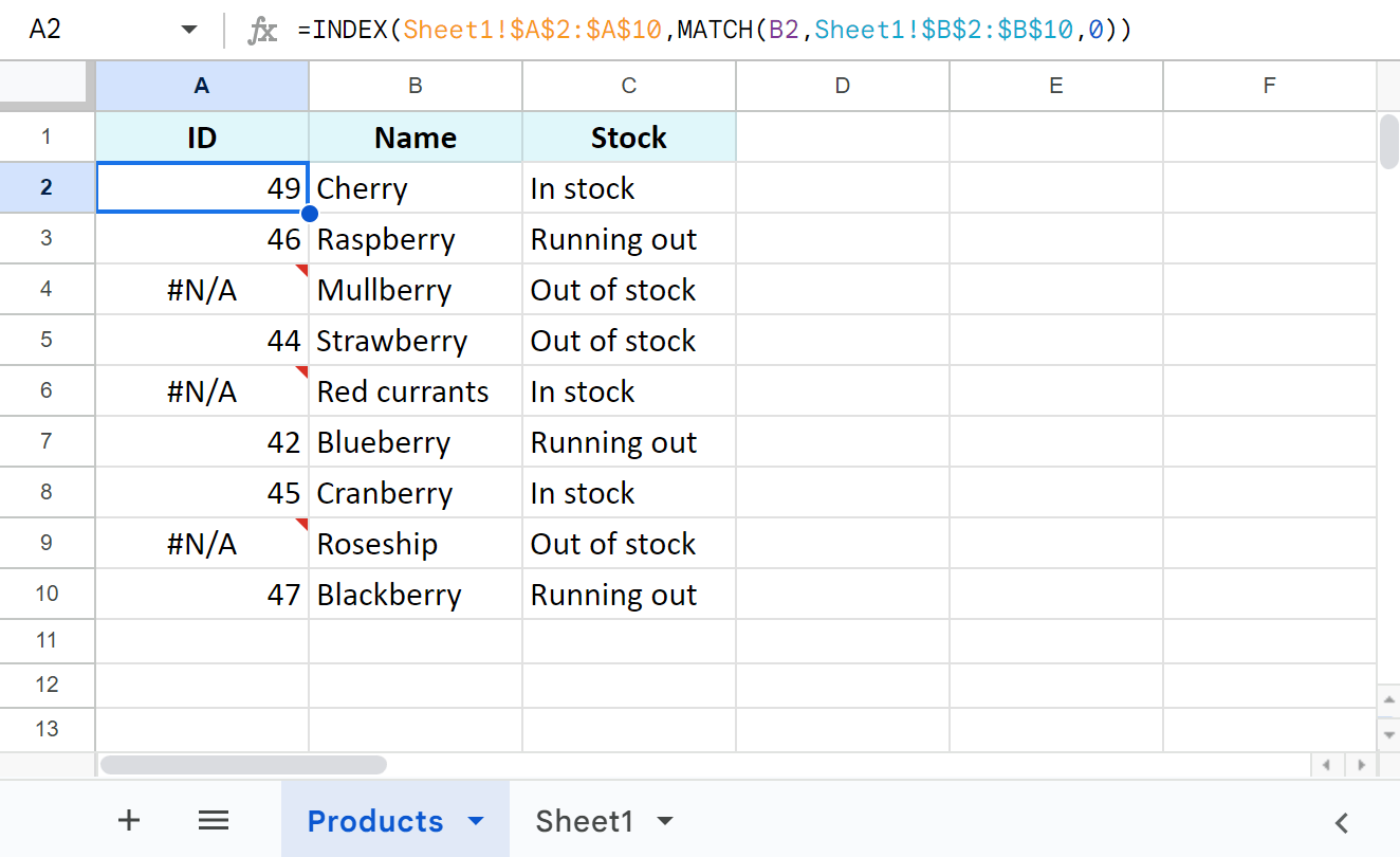
It works just like the first INDEX MATCH because it doesn't matter what column to look at. Easy-peasy :)
To fix those #N/A errors, once again, wrap INDEX MATCH in IFERROR:
=IFERROR(INDEX(Sheet1!$A$2:$A$10,MATCH(B2,Sheet1!$B$2:$B$10,0)),"")
Now, how do you use INDEX MATCH to merge those Google sheets and update all cells in the entire column at once?
Well… You don't. There's a little problem: ArrayFormula doesn't work with these two.
You will need to copy the INDEX MATCH formula down the column or use the Google Sheets QUERY function as an alternative.
3. Use QUERY to merge Google sheets & update cells
Google Sheets QUERY is the most powerful function in spreadsheets. So it's no surprise it offers a way to merge two or more Google sheets (match & update values).
Tip. If you've never used Google Sheets QUERY before, this tutorial will get you through its peculiar language.
Here's how the basic QUERY formula looks:
How do you use it to merge two sheets and update the Stock column with the actual data?
=QUERY(Sheet1!$A$2:$C$10,"select C where B='"&Products!$B2:$B$10&"'")
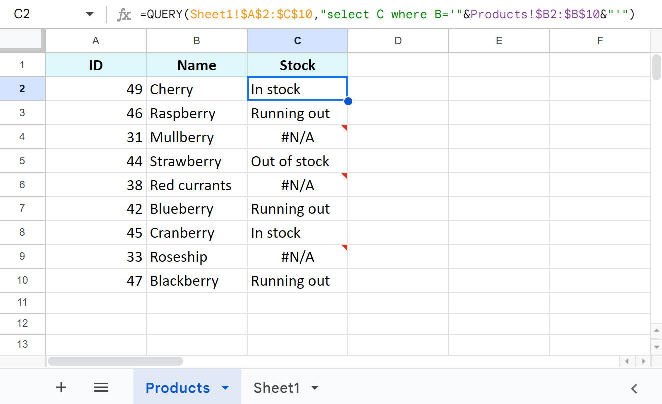
- Google Sheets QUERY looks at my lookup sheet — Sheet1 — since there are records I want to pull to my main table.
- And returns all those cells from column C only where column B matches berries in my main table.
Additionally, let me just lose those errors for cells without matches using IFERROR:
=IFERROR(QUERY(Sheet1!$A$2:$C$10,"select C where B='"&Products!$B2:$B$10&"'"),"")
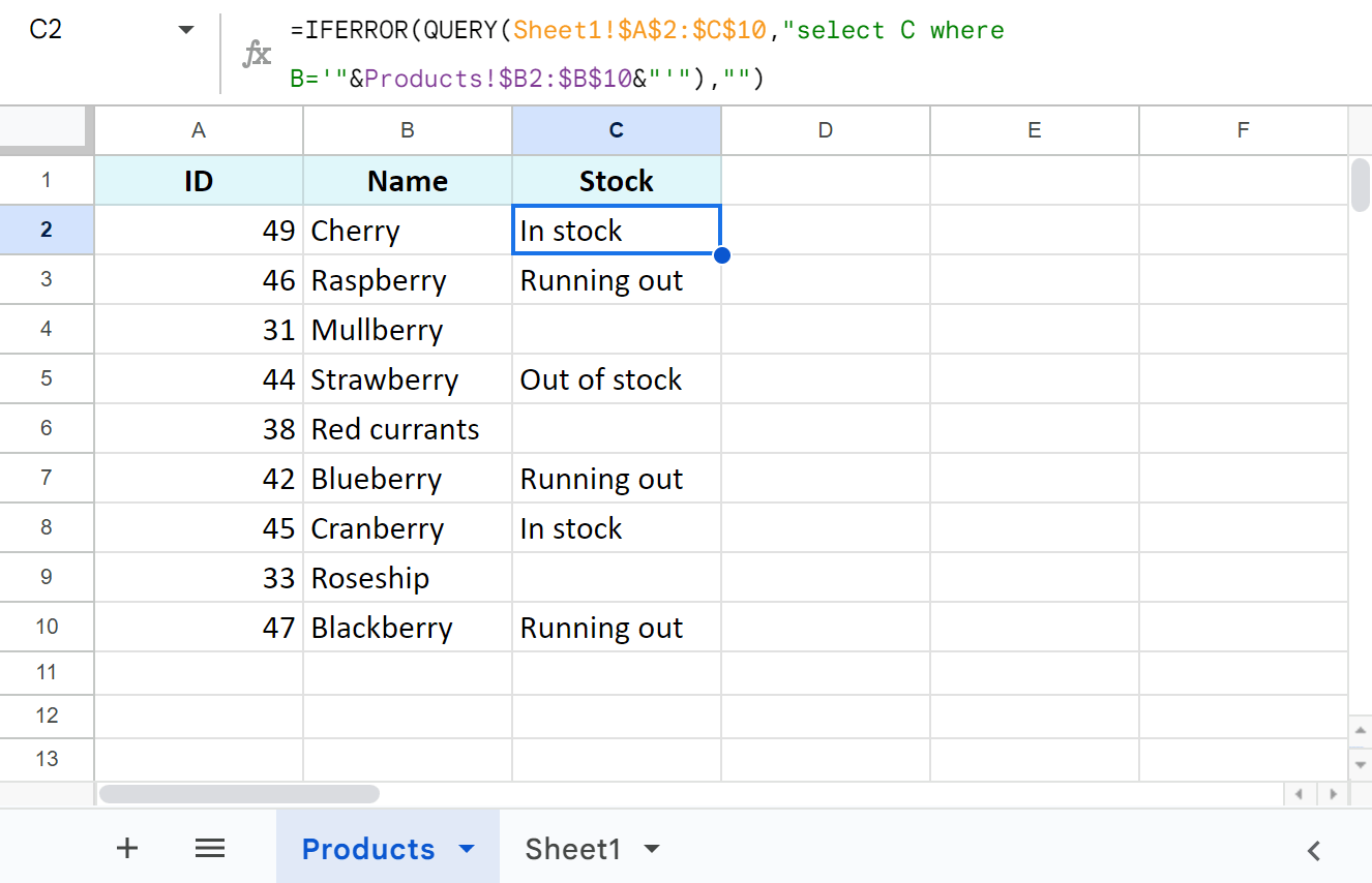
Well, that's better :)
4. Merge Google sheets from different files — IMPORTRANGE function
There's one more function I'd like to mention. It's important because it lets you merge multiple sheets even from different Google spreadsheets (files).
The function is called IMPORTRANGE:
- It starts with a link to a spreadsheet where you pull the data from (lookup spreadsheet).
- Followed by a sheet & a range that you want to take from that spreadsheet.
Note. I highly recommend going through Google docs on this function so you don't miss out on any important nuance of its work.
Imagine that your lookup sheet (with reference data) is in Spreadsheet 2 (lookup spreadsheet). Your main sheet is in Spreadsheet 1 (main spreadsheet).
Note. For IMPORTRANGE to work, you must connect both files. Google Sheets always suggests a button for that right after you enter your formula. You can learn more about it in this step-by-step guide.
Let's use IMPORTRANGE with each function you learned earlier to merge Google sheets from different files.
Example 1. IMPORTRANGE + VLOOKUP
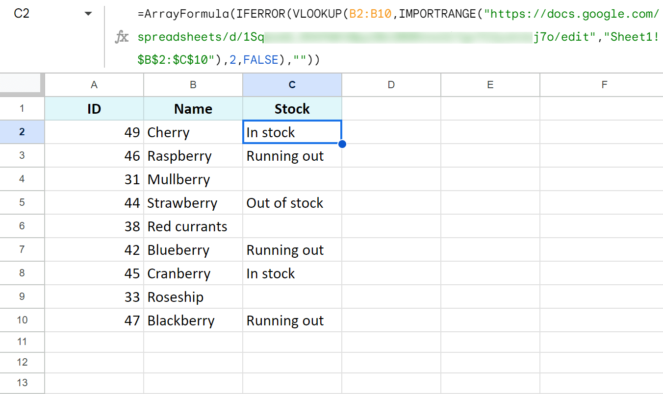
Use IMPORTRAGE as a range VLOOKUP to merge two Google sheets from different files:
=ArrayFormula(IFERROR(VLOOKUP(B2:B10,IMPORTRANGE("https://docs.google.com/spreadsheets/d/1Sq…j7o/edit","Sheet1!$B$2:$C$10"),2,FALSE),""))
Example 2. IMPORTRANGE + INDEX MATCH
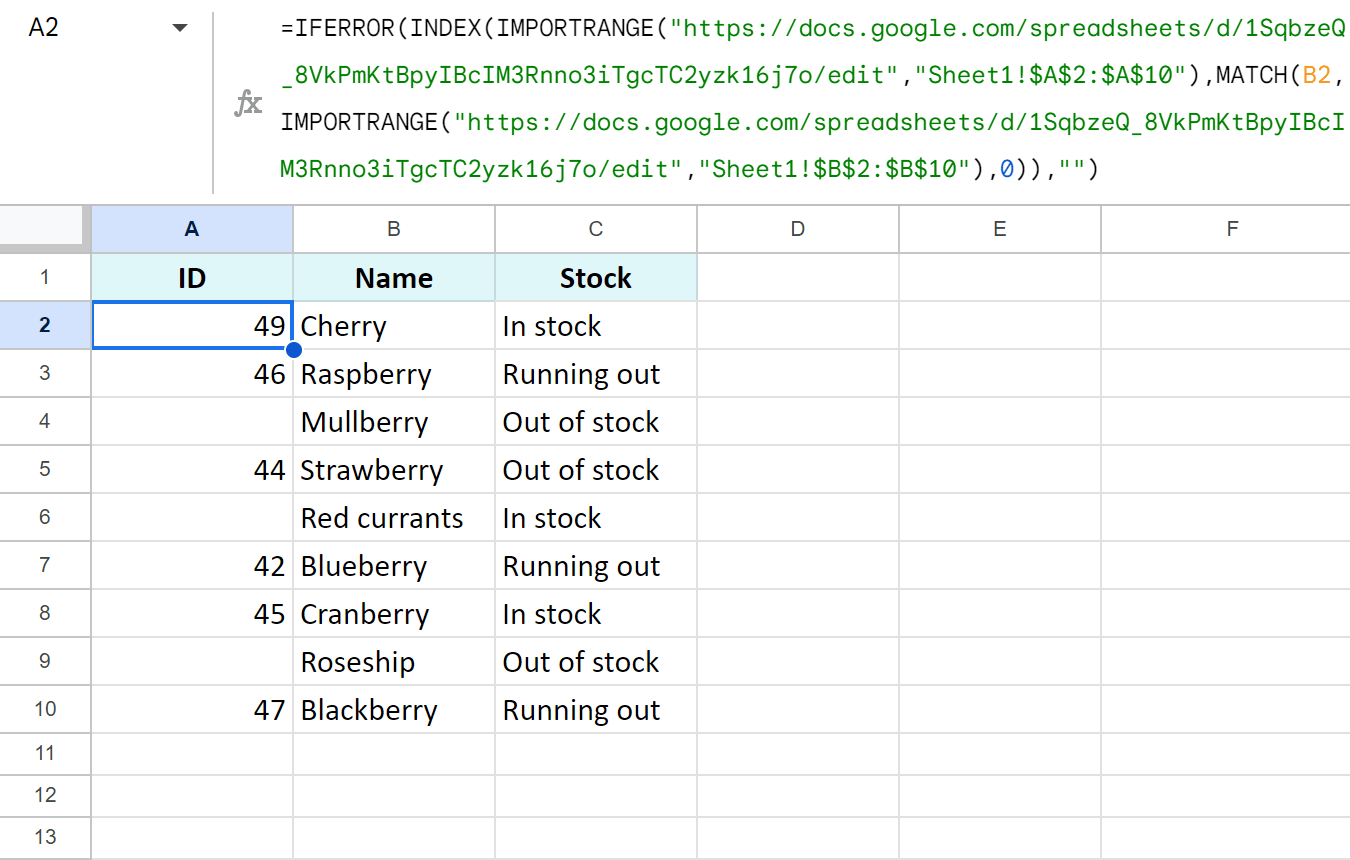
As for INDEX MATCH & IMPORTRANGE, you will need to reference another spreadsheet twice: as a range for INDEX and as a range for MATCH:
=IFERROR(INDEX(IMPORTRANGE("https://docs.google.com/spreadsheets/d/1Sq…j7o/edit","Sheet1!$A$1:$A$10"),MATCH(B2,IMPORTRANGE("https://docs.google.com/spreadsheets/d/1Sq…j7o/edit","Sheet1!$B$2:$B$10"),0)),"")
Example 3. IMPORTRANGE + QUERY
This tandem of formulas is my personal favourite. Togethe, they can deal with almost anything in spreadsheets when used together. Merging Google sheets from separate files is not an exception:
=IFERROR(QUERY(IMPORTRANGE("https://docs.google.com/spreadsheets/d/1Sq…j7o/edit","Sheet1!$A$2:$C$10"),"select Col3 where Col2='"&QUERY!$B2:$B$10&"'"),"")
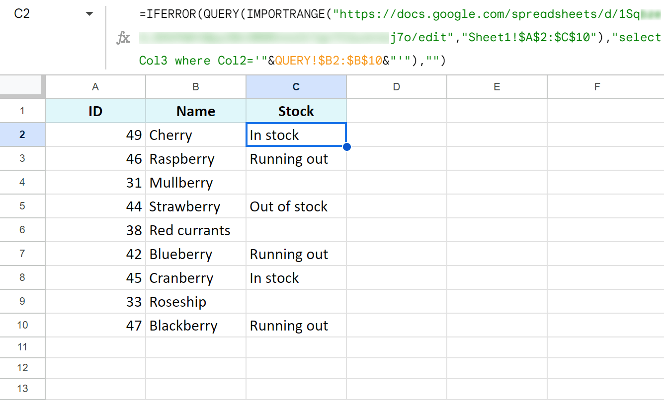
Voila :) That's all for functions & formulas. You are free to pick any function & build your own formula by the examples above…
or…
try a special tool that merges Google sheets FOR you! ;)
Easiest way to match & merge Google sheets — Merge Sheets add-on
If you don't have time to build or even learn formulas, or if you're simply looking for the easiest way to match and merge Google Sheets, Merge Sheets add-on is what you're looking for.
All you will need to do is tick off the checkboxes in 5 user-friendly steps:
- select your main sheet
- select your lookup sheet
- tick off key columns (those that should match)
- choose columns to update and/or add:
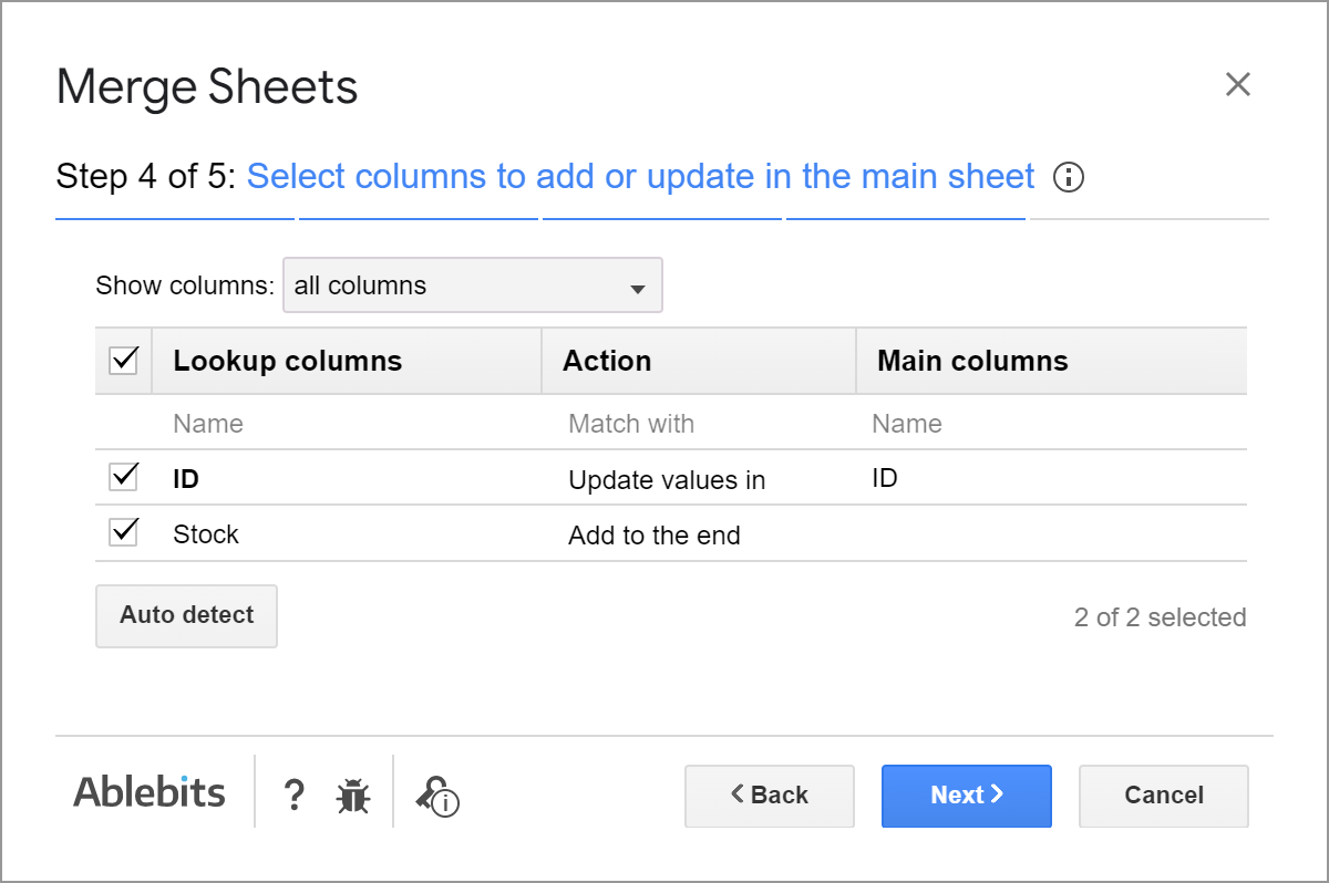
- adjust additional options, e.g., where to place the results, or color updated records, or mark them in a status column, etc.
- click Merge
Once the add-on does the job, it will even offers to save this run into a scenario. You will be able to reuse it from the Google Sheets menu in a click whenever you need:
Watch this 3-minute demo video to see how Merge Sheets add-on works: 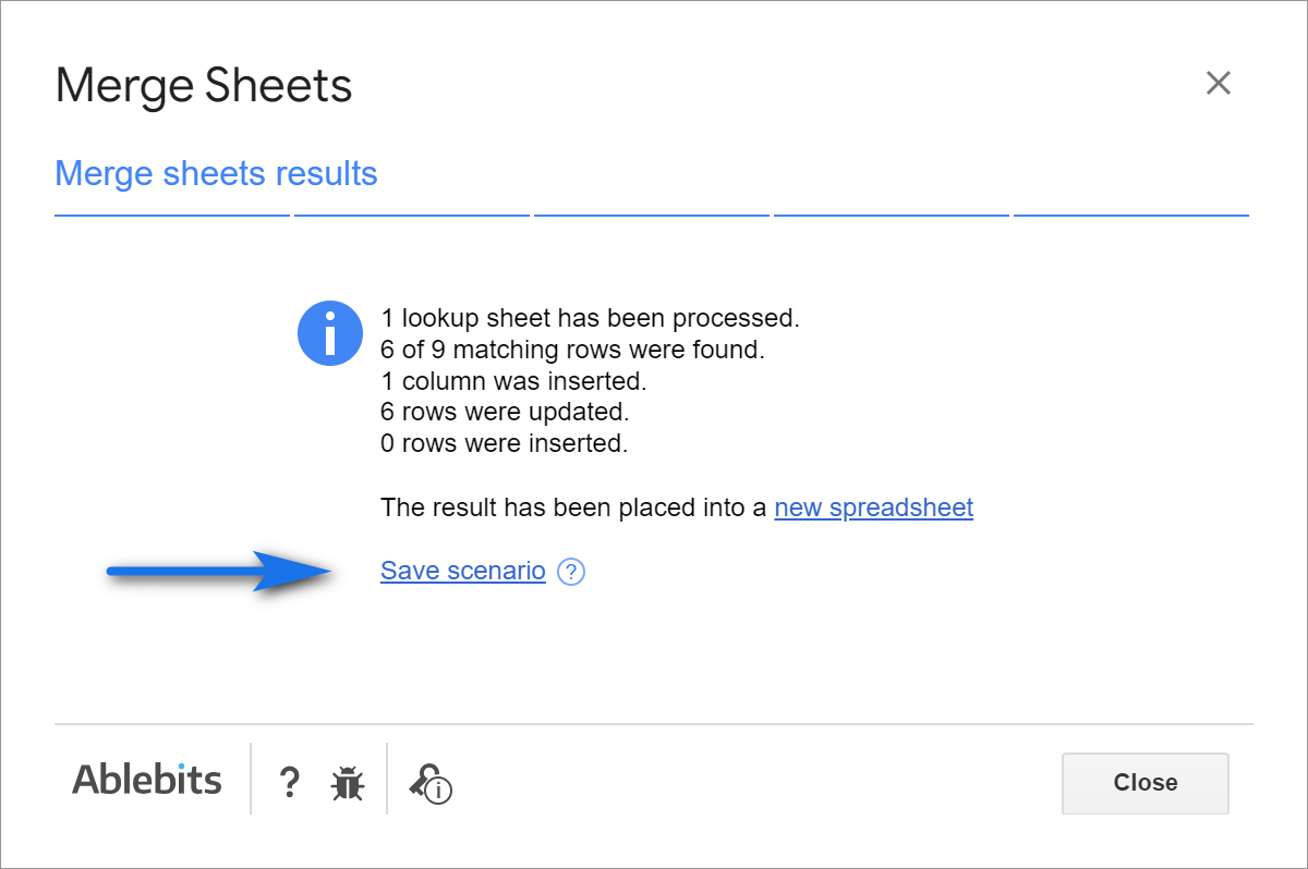
Video: Easiest way to merge Google sheets
I encourage you to install Merge Sheets from the Google Sheets store and follow these instructions to match and merge your tables. And let me know how it goes in the comments section!
Spreadsheet with formula examples
Merge Google sheets & update data - formula examples (make a copy of the file)
 by
by
6 comments
I am trying to build a script where a document is created for every row in a sheet where there is an unknown number of rows in the sheet. The sheet was created by Forms and continues to grow as replies are recorded. My script works great to create the documents but keeps on running creating blank documents until I Cancel the script. How do I end the execution once the end of the data is reached?
function createNewGoogleDocs() {
//This value is the id of the document template
const googleDocTemplate = DriveApp.getFileById('XXXXXXXXXXXXXXXXXXXXXXXXXXXXXXXXXXXX');
//This value is the id of the folder where completed documents are stored
const destinationFolder = DriveApp.getFolderById('XXXXXXXXXXXXXXXXXXXXXXXXXXXX')
//Here we store the sheet as a variable
const sheet = SpreadsheetApp
.getActiveSpreadsheet()
.getSheetByName('Comparrison')
//Now we get all of the values as a 2D array
const rows = sheet.getDataRange().getValues();
//Start processing each spreadsheet row
rows.forEach(function(row, index){
//Here we check if this row is the headers, if so we skip it
if (index === 0) return;
if (index === 1) return;
//Here we check if a document has already been generated by looking at 'Document Link', if so we skip it
if (row[53]) return;
//Using the row data in a template literal, we make a copy of our template document in our destinationFolder
const copy = googleDocTemplate.makeCopy(`${row[0]} Health Status Summary` , destinationFolder)
//Once we have the copy, we then open it using the DocumentApp
const doc = DocumentApp.openById(copy.getId())
//All of the content lives in the body, so we get that for editing
const body = doc.getBody();
//In these lines, we replace our replacement tokens with values from our spreadsheet row
body.replaceText('{{Email Address}}', row[0]);
body.replaceText('{{Digestive Track Before}}', row[1]);
body.replaceText('{{Digestive Track After}}', row[2]);
body.replaceText('{{Digestive Track Delta}}', row[3]);
etc etc
//We make our changes permanent by saving and closing the document
doc.saveAndClose();
//Store the url of our new document in a variable
const url = doc.getUrl();
//Write that value back to the 'Document Link' column in the spreadsheet.
sheet.getRange(index + 1, 54).setValue(url)
})
}
Hello Jack,
We're always ready to help you, but we do not cover the programming area (script-related questions).
You may try to find a solution here – an overview of Google Apps Script with a lot of helpful content and links:
https://developers.google.com/apps-script/overview
I hope you’ll find this information helpful. Sorry I can't assist you better.
Hello
I tired =IMPORTRANGE("spreadsheet_url","range_string") but it can only import the first sheet of the workbook.
Is there a way to import the second page onwards?
Hello Lvna,
For the "range_string", you need to specify the name of the required sheet along with the range. Please look through formula examples in this part of the article or this step-by-step tutorial on building IMPORTRANGE formulas.
Hi,
I am currenty using a query formula to pull through data from one sheet onto another sheet based on a set criteria but also where one piece of data in column A on the sheet the data is being pulled into and also has a to match one piece of data in the other sheet in column A ( this piece of data changes on each row in both sheets)
I am currently using the below formula but they last command where A matches '"&A:A&"' is not working.
=IFNA(QUERY('Data Dump'!$A$1:$Z,"select Q where A is not null and M matches '"&L$2&"' and A matches '"&A:A&"' ",0),"")
Is this possible within a query formula and if so what amends do I need to make to my existing formula.
Thanks you so much for your time and help.
Best wishes
Emily
Hi Emily,
For me to be able to help you better, please share an editable copy of your spreadsheet with your formula with us: support@apps4gs.com. Please include the example of the result you expect to get.
If you have confidential information there, you can replace it with some irrelevant data, just keep the format.
I'll look into it and try to help.
Note. We keep that Google account for file sharing only and don't monitor its Inbox. Please do not email there. Once you share the file, just confirm by replying to this comment.