Concatenate usually means to link something together in a series or a chain. It's what you do whenever you merge text from multiple Google Sheets cells. This article collects the most popular and easy solutions to help you solve the concatenation puzzle.
However big your dataset is, you may come across the task of combining multiple cells in Google Sheets together. And I have no doubt you will want to not only keep all values from losing, but also add some commas, spaces, or other characters, or even separate those records with other text.
Well, spreadsheets offer several tools for this task.
Google Sheets CONCAT function
The CONCAT function is a simplified version of Google Sheets CONCATENATE:
To join cells with this function, you need to list the required values:
- value1 — a record to which value2 should be appended.
- value2 — the value to join.
To get one string from 2 text or numeric units, the formula will look like below, with each record in double quotes:
=CONCAT("2019:","The Lion King")

In reality, your data is most likely already in cells. You can refer to those cells directly instead of putting down each number or text as an argument. So the real-data formula will be like this:
=CONCAT(A2,B2)
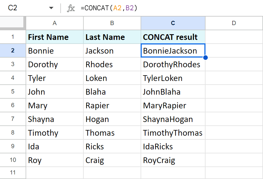
Tip. To copy your formula to the whole column, select the cell with the formula and double-click the little square at the bottom right corner of the cell. The formula will automatically fill the entire column adjusting all cell references, till the end of the table.
As you can see, the function is super simple, but it has major weak points:
- it merges only two cells in Google Sheets at a time.
- it cannot combine columns, rows, or or other large data sets, it takes only single cells. If you try to merge multiple cells, the formula will either return an error or join only the first two values, like this:
=CONCAT(A2:A11,B2:B11)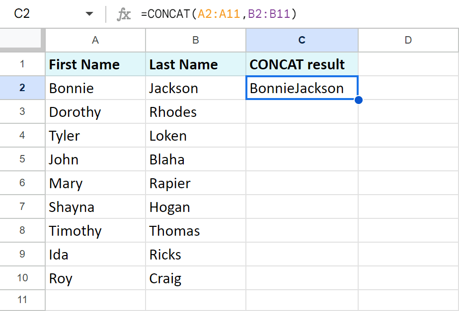
CONCAT alternative: concatenation operator ampersand (&)
Formulas always need lots of different operators for various purposes. Concatenation is not an exception. Using an ampersand character (&) in formulas instead of the CONCAT function will provide you with the same result:
=A2&B2
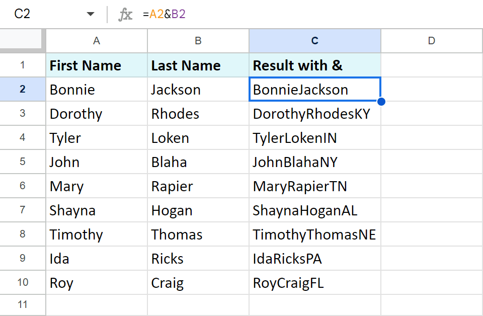
But little do you know that this concatenation operator is more flexible. Here's what it can do:
- Merge more than two values at a time:
=A2&B2&C2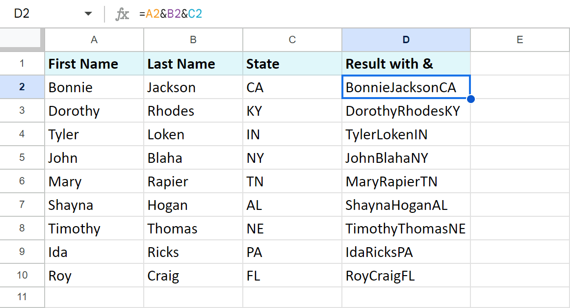
- Not just merge cells in Google Sheets, but also separate them with various characters:
=A2&" "&B2&"; "&C2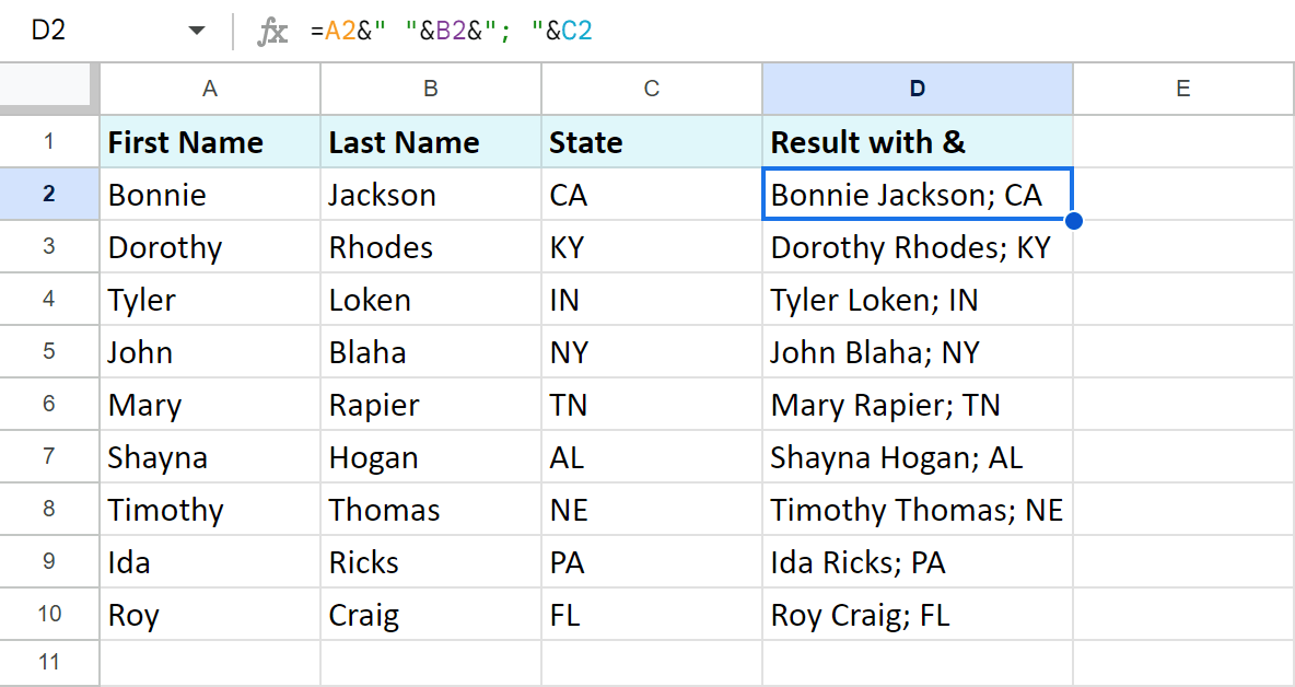
If you still don't get the desired result with these options, there's one more function to try.
How to use CONCATENATE in Google Sheets
I believe Google Sheets CONCATENATE function is the first one you will use to merge cells.
CONCATENATE text strings and numbers in Google Sheets
The formula pattern consists of the following arguments:
- string1 is the first string you want to append other values to. This argument is required.
- string2, … stands for all other strings you may want to append. This argument is optional.
Note. The outcome record will consist of the strings in the order of their appearance in the formula.
If I adapt the formula to my data, I will get this:
=CONCATENATE(A2,B2,C2)
Or, since the function accepts ranges:
=CONCATENATE(A2:D2)
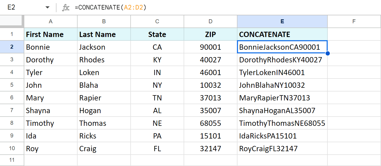
You can immediately notice the first advantage of Google Sheets CONCATENATE: it easily joins over two cells with both text and numbers.
Google Sheets: concatenate strings with separators
Combining cells in Google Sheets is half the work. But to make the result look pretty and readable, you should add some extra characters.
If you keep the formula as is, it will just glue everything together: BonnieJacksonCA, BonnieJacksonIN, etc. But Google Sheets CONCATENATE takes characters as arguments, too.
Thus, to add some separators for readability, mention them in double quotes in the formula:
=CONCATENATE(A2," ",B2,", ",C2)
Here I want to concatenate A2 & B2 with space and separate B2 from C2 with a comma and space:
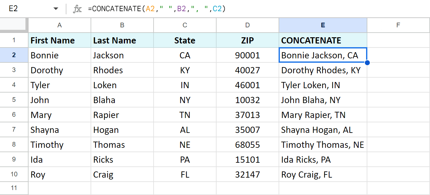
You are free to use almost any character in the function like this, yet a line break requires a different approach.
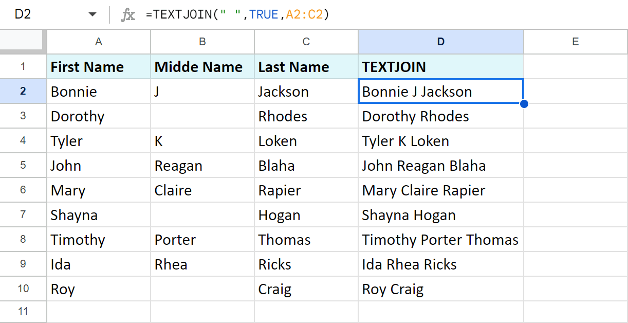
Tip. In case there are empty cells in some of the columns you're merging, there's one more function you may be interested in. TEXTJOIN not only merges cells in Google Sheets but also ignores blanks:
=TEXTJOIN(" ",TRUE,A2:C2)
Here's how it works:
- Indicate the desired delimiter as a first argument — space (" ") for me.
- Put TRUE as a second argument to skip blank cells or FALSE to include them in the result.
- Enter the range to merge.
Concatenate with line break in Google Sheets
While it's obvious how to enter most delimiters to the function, you cannot type a line break the same way there. But luckily Google lets you play many different cards.
One of them is a functions called CHAR. It helps get various special characters. You see, each character has a place in the Unicode table. You just need to feed the ordinal number of the character from that table to the function and the latter will return the character itself.
Here's a formula to get the line break:
=CHAR(10)
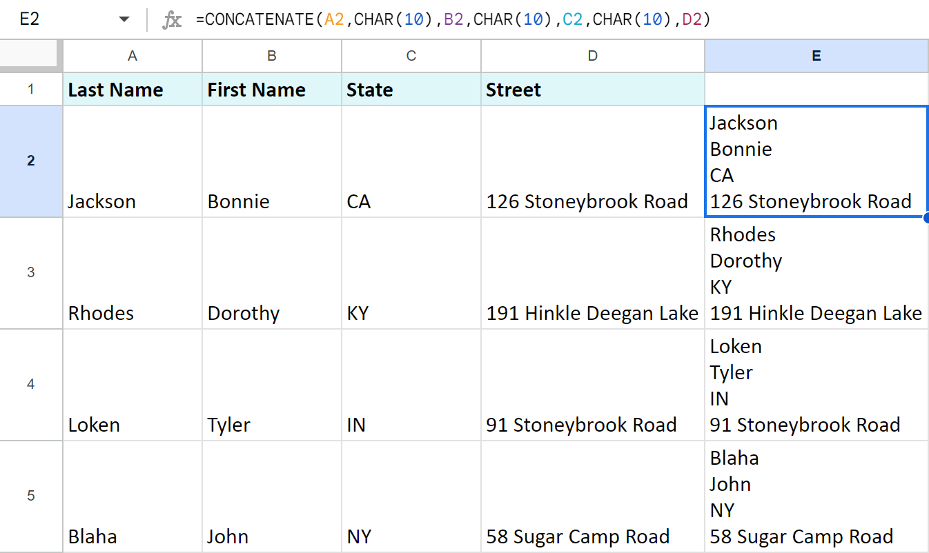
Add it to the formula to concatenate with the line break in Google Sheets:
=CONCATENATE(A2,CHAR(10),B2,CHAR(10),C2,CHAR(10),D2)
Combine date and time in Google Sheets
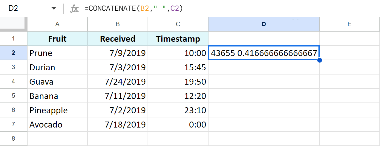
If you try to combine date and time in Google Sheets using one of the methods above, it won't work. Your spreadsheet will return numbers:
To merge cells in Google Sheets with date and time units correctly, use the TEXT function:
- where number is any number, date, or time you'd like to get in the desired format
- and format is the pattern you'd like to see as a result.
Tip. In my example, I'm going to reference cells with dates and times, but you are free to use date/time units or even such functions as DATE or TIME directly in the formula.
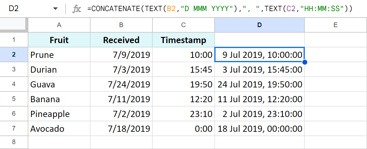
- I use the first TEXT formula to change the date format from 7/9/2019 to 9 Jul 2019:
=TEXT(B2,"D MMM YYYY") - The second TEXT returns the time:
=TEXT(C2,"HH:MM:SS") - Using these in CONCATENATE, Google Sheets lets me combine date and time in the desired format with other characters or text:
=CONCATENATE(TEXT(B2,"D MMM YYYY"),", ",TEXT(C2,"HH:MM:SS"))
How to merge columns in Google Sheets
With slight adjustments, all the ways I mentioned are capable of merging columns in Google Sheets.
Example 1. Google Sheets CONCAT
To merge whole columns in Google Sheets with CONCAT, select the entire range that should contain the result (C2:C11 in my case) and enter your formula wrapping it in ARRAYFORMULA:
=ARRAYFORMULA(CONCAT(A2:A10,B2:B10))
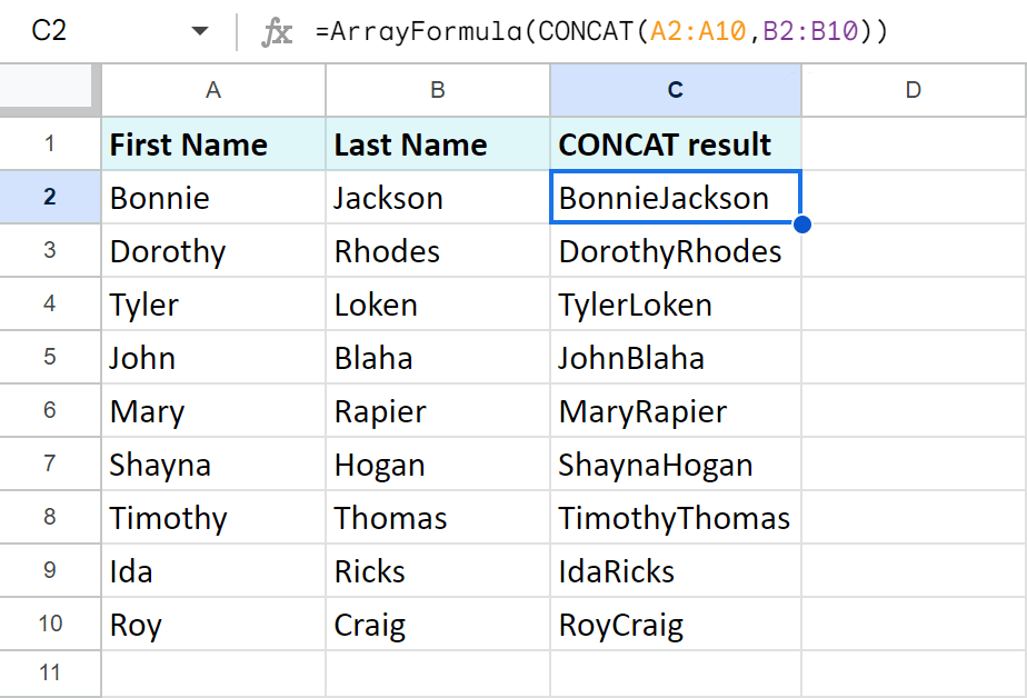
Note. You could use the CONCATENATE function, but it will join all records within one cell since it easily merges multiple cells and data ranges.
Example 2. Concatenation operator
Create array formulas to merge columns in Google Sheets using the ampersand and add separators at the same time:
=ARRAYFORMULA(A2:A10&" "&B2:B10&"; "&C2:C10)
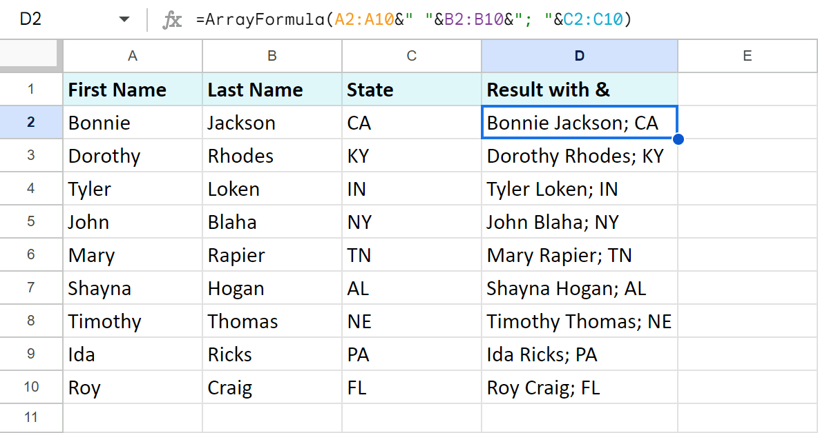
This looks good, but I have to mention some major cons.
Listing all columns if you have too many of them can become a pain in the neck, especially if you accidentally skip/duplicate/mix up any characters.
Also, if you decide to add more columns to the formula later, you'll have to edit every existing range in the formula manually.
The next example solves these problems.
Example 3. Google Sheets QUERY
Google Sheets QUERY function is also suited to merge several columns in Google Sheets. Have a look:
=TRANSPOSE(QUERY(TRANSPOSE(A2:D10),,9^9))
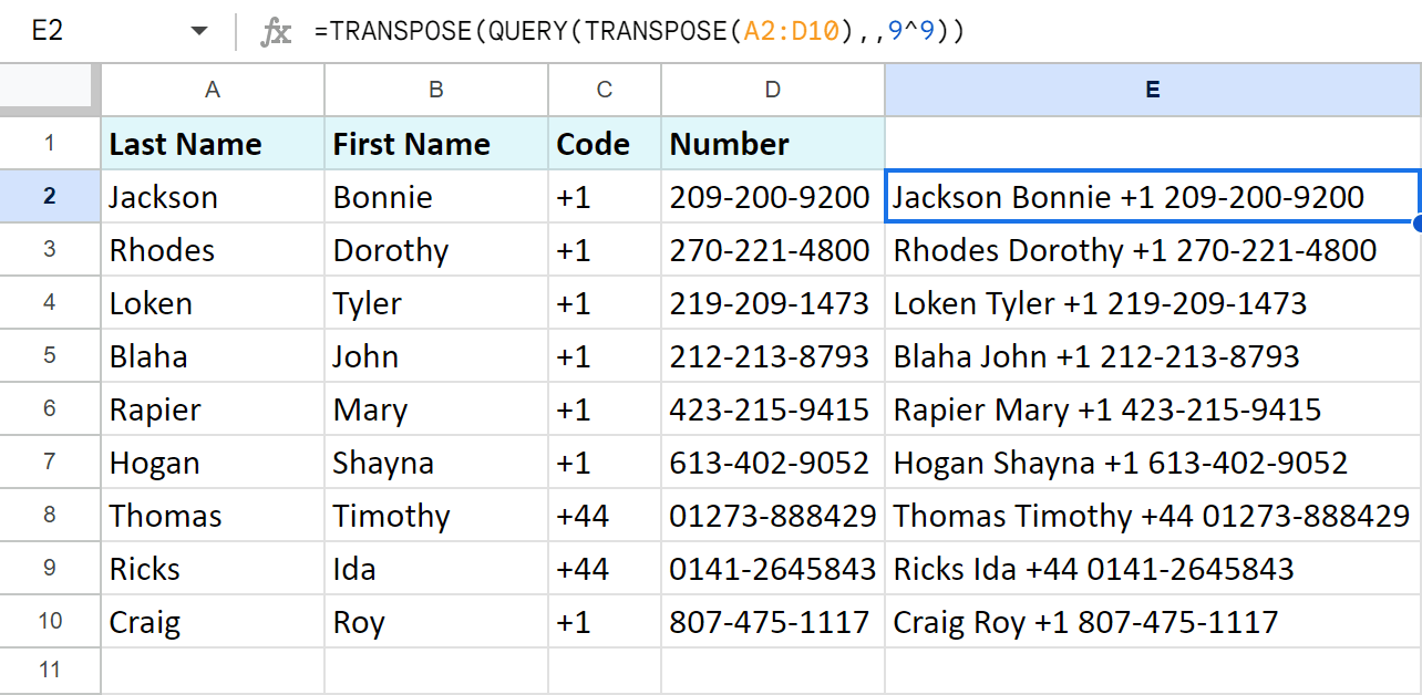
You may think this strange formula is beyond your grasp, but let me lay its all pieces out for you:
- =TRANSPOSE(A2:D10) turns the rows of data into columns.
- =QUERY(TRANSPOSE(A2:D10),,9^9) merges records in each column to the top cells.
Tip. When I put 9^9 into the formula, I tell that formula to pull all rows from all columns into the first row as if they were headers. 9^9 expression includes all possible cells in the spreadsheet (remember the limit for 10M cells?) and is easy to remember :)
- =TRANSPOSE(QUERY(TRANSPOSE(A2:D10),,9^9)) takes that header row from QUERY and turns it into a column like the one I've got.
Here are the perks of merging columns in Google Sheets using QUERY:
- you don't need to select the entire column as you do for array formulas
- only need to mention each column in the formula if they are non-adjacent. In this case, here's how the formula will look:
=TRANSPOSE(QUERY(TRANSPOSE({A2:A10,C2:C10,E2:E10,G2:G10}),,9^9))
How to merge cells in Google Sheets without formulas
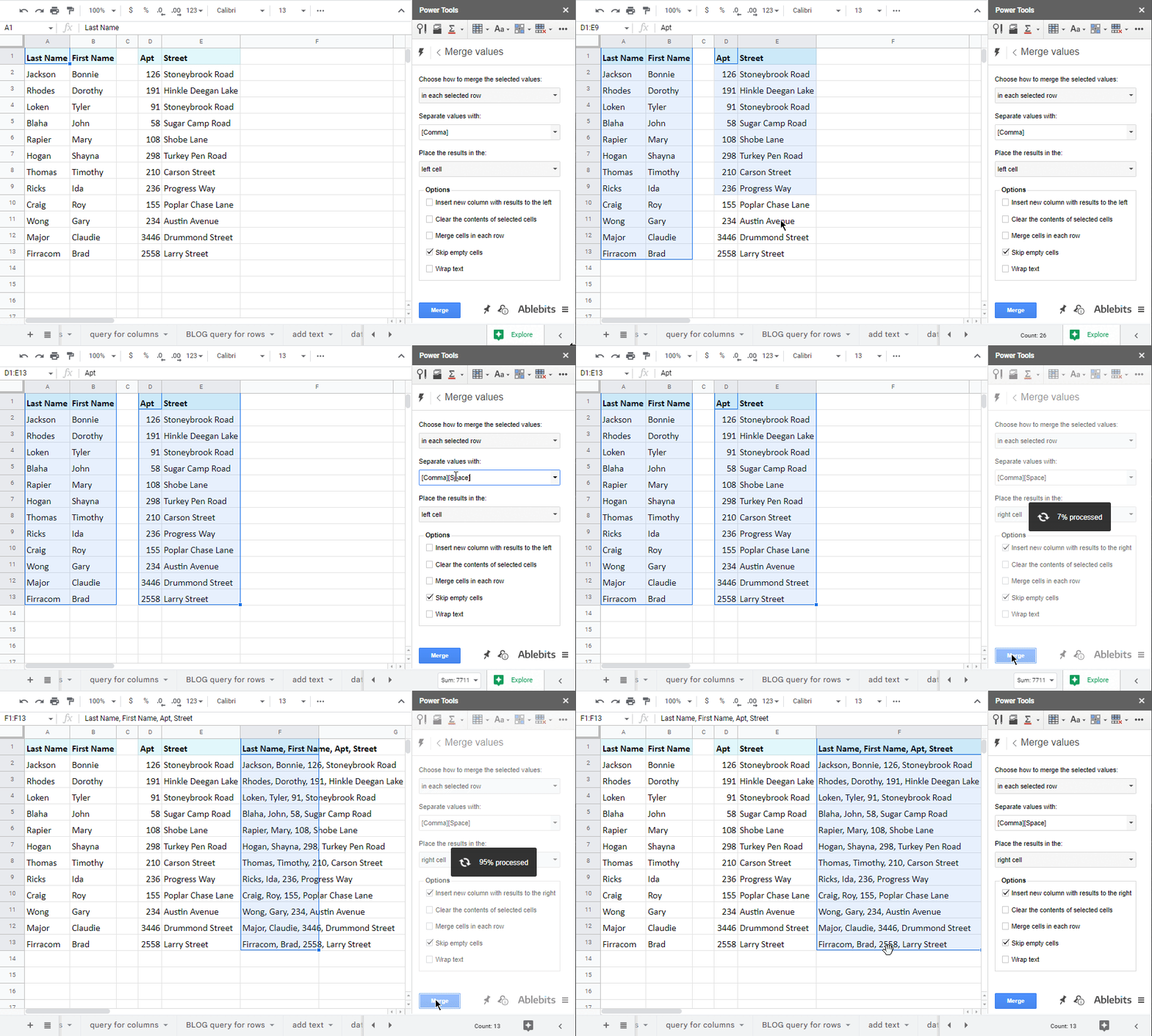
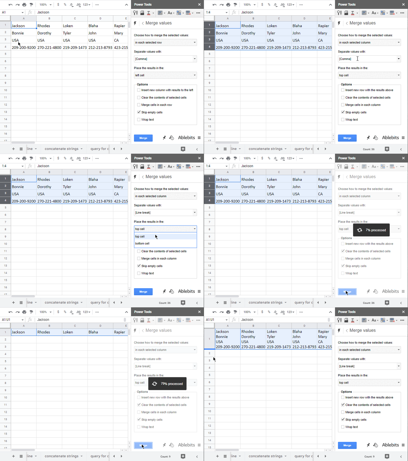
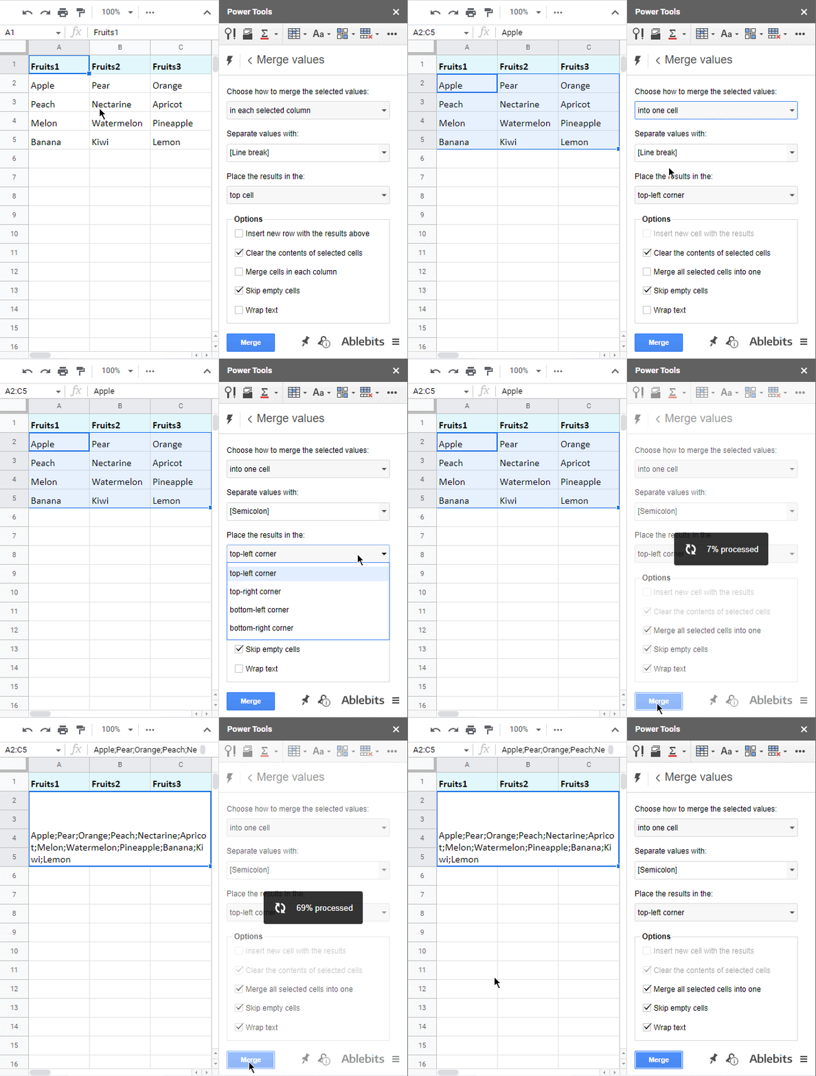
If mastering different formulas is not part of your plan, you will benefit from our Merge Values add-on. It quickly combines columns in Google Sheets as well as rows and other ranges. Even non-adjacent ones! Its options are crystal clear, and all you have to do is select the range and decide on how the result should look.
- You can choose to merge columns in Google Sheets — even non-adjacent ones, separate them with commas and spaces, and place the result to the right of the original records:
- Or merge rows in Google Sheets, divide records with line breaks, and clear the contents of selected cells:
- Or select the range and combine all cells in Google Sheets into one altogether:
If you're interested in this Google Sheets app, you can look through everything it does on this special page or in this short video tutorial:
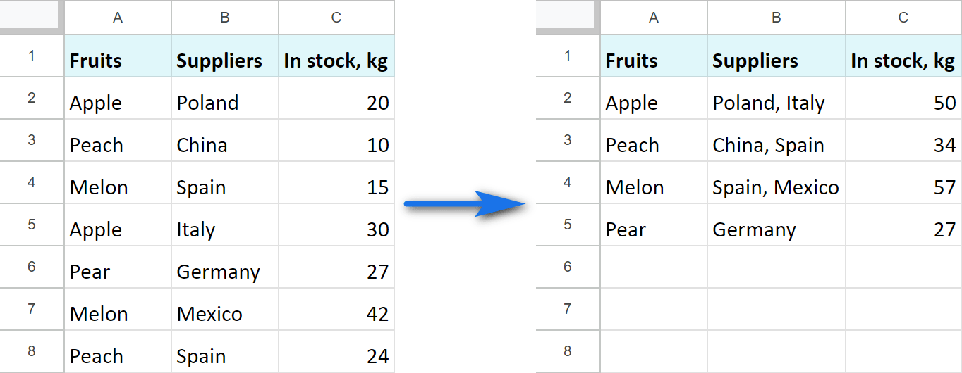
- There's one more utility to concatenate in Google Sheets — Combine Duplicate Rows. On one hand, it merges duplicate rows by key columns. On the other hand, it tallies numbers that belong to the same record:
Learn how to use Combine Duplicate Rows in this video:
Concatenate and add text by position
You already know that you can add missing text, numbers, and characters to your strings using the CONCATENATE function.
Tip. See more formulas on that in this tutorial.
But if there are too many records to join, any extra characters can extend your formula way beyond what you have planned. In cases like this, it's better to merge cells in Google Sheets as they are or use simple delimiters like space and add the text after that. A special tool of ours will help you.
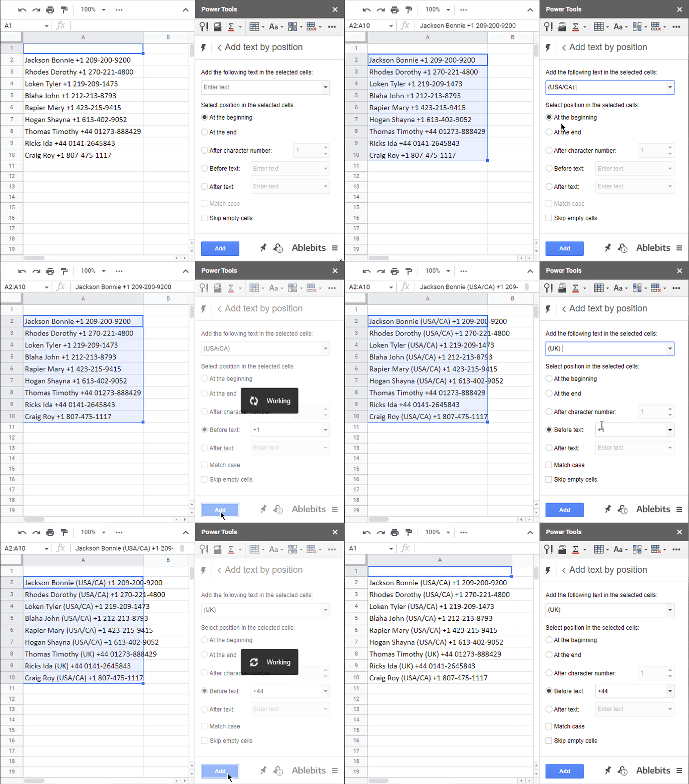
Add text by position inserts any chars and strings by the position you specify. Without formulas :) Let me show you how it works.
In the previous example QUERY joined names and phone numbers for me. But I'd like to add country short forms: (USA/CA) before phone numbers that start with +1 and UK before +44:
`
I hope by now you've decided which of the ways suits your case best. If you have any other methods in mind, please do share with us in the comments section below :)
 by
by
37 comments
Hi Natalia
Thanks for all of your excellent answers!
I want to combine the content of two columns in a third column with a space between the data, and have figured out how to do that.
But I would like to eliminate this combination if one of the cells in the original two columns is blank.
How, pretty please?
Thanks so much
Marc
Hi Marc,
Thank you for your feedback!
For me to be able to help you better, please specify the exact formula you're using to combine the data with a space in between.
I have a google sheet with behavior data by grade (K-12). I'm trying to make a bar graph with the number of behaviors for each grade. My bar graph has the numeral grades, but not the K for Kindergarten. Is there a way to get it to include the kindergarten data too?
Thanks
Hello Ruth,
Please refer to this article regarding charts in Google Sheets. If you still need help after looking into it, please consider sharing an editable copy of your spreadsheet with us (support@apps4gs.com) with a description of your task AND your current chart. I'll try to help.
Hi Natalia,
What is the concatenate formula to include unit separator? Example: cell 1: 12000, cell 2: sheets. Expected answer: 12,000 sheets
Hi Yim,
Since 12,000 is merely a displayed format, you need to concatenate using the format as well:
=CONCATENATE(TEXT(A1,"#,###")," ",B1)
Hello, I have a small problem in preparing some data for import into a database. My current format is 3 rows -
Row 1 - Product number
Row 2 - Link where the image is located
Row 3 - I have the number of images
Thus, if the product has only one image in the third row, it is the number 1, if the product has 2 or more images, it has the next number in the next row, for example. ( Product 1 - Link - 1 ) row 1 , ( Product 2 - Link - 1) row 2 , ( Product 2 - Link - 2 ) row 3 ..........( Product 2 - Link - 10 ) row 10
Now the database receives multiple image link values for each product if they are passed in a single cell and the links are separated by " ,"
As I have somewhere around 800,000 values, I wonder if there is somehow a formula to be able to join the links with the appropriate format for importing into the database
I'm attaching a link from Google Shetts so you can better understand what formula I need -
Thank you in advance for any help
https://docs.google.com/spreadsheets/d/1ci9qvDaklt0WdURe8mlBOlYvVEcM_cXzyYVom7gFOKo/edit?usp=sharing
Hello Ion,
I'm sorry but I don't have access to your spreadsheet. If you still need help, please share it directly with support@apps4gs.com and let me know here in the comments once you do. Please also make sure the example of the expected result is included. I'll do my best to help.
Thanks for the cool tutorial! However, I'm getting crazy over one problem: concatenate adds additional double quotes to existing ones when copying data out merged text, which is extremely annoying as the additional quotation marks are not visible in the merged text in google sheets.
For example, if you do this in A1: key=" and concatenate it with A2: value", CONCATENATE(A1:A2) will look like: key="value", but when you copy the contents from the concatenated cell, you will get: key=""value"". Is there any way around this?
Hello Bjoern,
I'm sorry, the problem doesn't appear on my end. Could you please specify what you click/press to copy and paste that concatenated value? I tried to paste it as a value, and the result looks ok: key="value"
Hi! I'm trying to combine plant data from a spreadsheet to use on a website. I need to combine the genus and species, add some formatting, and land everything including the correct formatting into a single cell. I could use google sheets or Excel, don't really care which. But, concatenate and the "&" function strip formatting.
For example, I start with column C, the genus "Acer" (italicized) and column D, the species "negundo" (also italicized), add in parenthesis around column D, common name "Boxelder" and I want this: Acer negundo (Boxelder), but with "Acer negundo" italicized, "Boxelder" not. (Sorry, your comment box doesn't let me format either so it's a little wordy here. Any way to help?
The formula is
=CONCATENATE(C3," ",D3," (",E3,")")
If I can't retain formatting there's no point in using a formula; we'll have to have a volunteer copy and paste each of these or highlight part of each cell and italicize.
Hi!
You can't retain formatting of each cell when merging the values of those cells.
Natalia, thank you for the article.
I have a related question. I needed to combine 7 columns and if a cell contains a particular data (e.g. "Apple"), to produce a note (e.g. "Attention") in the cell instead of combining cells. I found the explanation that IF function can help ().
Are there any options for this?
Would appreciate your reply and sorry for a noob question :)
Thank you for your feedback, Dima :)
I'm afraid there's no other way since IF is the only function that can test a cell against criteria and return a related value. We have a nice article explaining how it works, feel free to take a look: https://www.ablebits.com/office-addins-blog/if-function-google-sheets/
Heyy i want to merge or combine some column into one column, but the problem is that the columns that i want to merge is separated randomly with the same header names let's say "Fun Games #1". Is there any ways to combine them?
Hi Daniswara,
I'm afraid you'll need to do that in two steps with two formulas:
Thank you. I have a question for Example 3. Google Sheets QUERY using this formula " =TRANSPOSE(QUERY(TRANSPOSE(A2:D10),,9^9)) ". Is there any way to merge the rows using specific symbol or text? So if I split it again, I'll have a reference? thank you so much.
Hi Eric,
To merge rows from a column rather than columns from a row, use a formula like this:
=ArrayFormula(QUERY(A2:D10&CHAR(10),,9^9))
Hi I am not sure how to put this but I am trying to create myself a financial tracker of my personal finances and I am having a problem with tracking the Expenses in the dashboard... I used Query to get all of the descriptions in the input spreadsheet to the dashboard spreadsheet based on what categories and what month they are in. But... some of those descriptions are the same - for example "Grocery shopping Lidl" or just "Lidl" and those sometimes repeat as I go buy my groceries mostly to the same store :D but when I am tracking this I got let's say 5 different unique locations (descriptions) but totally like 20 items... My problem is... how do I merge them so they only show those 5 and combine them instead of listing 4x Lidl, 5x Aldi etc...
I am having a really difficult time with the power tool because it is only a part of the whole table and I would like to do it in query function if possible...
my query so far is this
=QUERY('TRANSACTIONS INPUT'!A:D,"Select C where (D='"&$H$7&"' and A ='"&$B$1&"') ",0)
Hi Jan,
For me to be able to help you better, please share a small sample spreadsheet with us (support@apps4gs.com) with 2 sheets: (1) an example of your source data (2) the result you expect to get (the result sheet is of great importance and often gives us a better understanding than any text description). I kindly ask you to shorten the tables to 10-20 rows. Please also include the QUERY formula you're trying to use.
Note. We keep that Google account for file sharing only and don't monitor its Inbox. Please do not email there. Once you share the file, just confirm by replying to this comment.
Hello,
My issue is to concatenate (op.gtin13 = "0000768000724" )
the number 0000768000724 being in the middle column, when I concatenate the result is:
(op.gtin13 = "768000724" ) but I need the 0s...
Could someone help me ?
Thank you in advance!!
Elena
Hello!
You haven't written what values you combine. You can put a zero in front of the number if the number is written as text, if the format is set to "text". You can add 0000 to each number if you use the custom number format "0000##; -0000##"
Please can someone help me, I want to make an inquiry reference automatically generated once the form is submitted through google forms
Hello Rameez,
for us to be able to suggest anything, please describe your task in detail.
Thank you for getting back to me and I apologize for not being more clear in my description. I'm combining First Name, Middle Initial, Last Name on a spreadsheet but there are a few instances that the person doesn't list a Middle Initial. When that happens the formula doesn't work. Is there a command that I can put in the formula that will fix this?
Thank you for the description, Amy,
Assuming those names are in columns A:C and the names themselves start from the 2nd row, here's the formula for you to try:
=TEXTJOIN(" ",TRUE,A2:C2)
This is exactly what I was looking for. However, the formula doesn't know what to do if one of the cells doesn't have data. Is there a way to compensate for that? Kind of like ignore if blank?
I will definitely check out the your PowerTools add-in.
Hello Amy,
Glad to know this article is helpful :)
Could you please share the exact formula you're using and specify which part can meet blanks?
Had followed your formula : =CONCATENATE(A2,CHAR(10),B2,CHAR(10),C2,CHAR(10),D2)
Managed to merge the multiple columns in a single column but how can i add the column names in front for eg.
Last Name : Johnny
First Name : Bonny
State : CA
Street : 126, Stoneybrook Road
Hello MJ,
Just add those column names or references to them into the formula to see them in the result.
For example, assuming your table starts with A1, the formula below will return you the first two rows you mentioned:
=CONCATENATE(A1," : ",A2,CHAR(10),B1," : ",B2)
Thank you so much! you saved me!
Hello, I need to create a formula that says if cell A2 says "January" and cell B2 says "Gloves" then take the value shown in range H2:H600 and put the final value in cell N2. eventually the formula will be used to determine how many instances of gloves were ordered in January.
Thank you
Hello Shelagh,
If I'm getting your task correctly, you should use the IF function or even COUNTIF function for the task. The links I provided will open the corresponding articles for you to check out.
Hi, would like to know how to convert my cell in text plain after concatenate a lot of columns, without the formula, Justo to be able to move my entire column without loosing the information?
Thanks
Hi Sandra,
We have a couple of tools for the task:
Hi!
Thanks for all this great info. I'm not sure if what I'm trying to do can be done in one formula or if it will take a few steps. I have events being submitted by a Google form and would like to merge the time data from the two cells (start time and end time) to a very specific format in a single cell. You'll see below, the format changes if both times are in the morning or afternoon, if they span noon, or if there are minutes to be included. If it's on the hour, I don't want :00 in the formatting and the a.m. or p.m. needs to be lower case with the periods. Examples:
- If the event starts and ends on the hour and in the same half of the day: 9-11 a.m. OR 6-8 p.m.
- If the event spans noon and is on the hour: 9 a.m.-3 p.m.
- If the event start or end time is during the hour: 9:30-11:45 a.m. OR 8:45 a.m.-4:15 p.m.
- Also, some of the above mixed: 9:15 a.m.-3 p.m. OR 10-11:30 a.m. OR 11 a.m.-3:45 p.m.
I plan to retain the original data columns for sorting.
Thanks for considering if you're willing to tackle this!
Hi there,
Thank you for your comment!
I'm afraid the task is not entirely clear. Please consider sharing a small sample spreadsheet with us (support@4-bits.com) with 2 sheets: the example of the source data and the result you expect to get. I kindly ask you to shorten the tables to 10-20 rows.
Note. We keep that email for file sharing only and don't monitor its Inbox. Please do not email there. Once you share the file, just confirm by replying here. We'll look into it and see if there's an easy solution.
In the meantime, try checking out these articles, you may find some useful and related info there:
IF function in Google Sheets
Date and time in Google Sheets
Calculate time in Google Sheets