Today I'm going to bring Google Sheets formulas to the table. I'll start with elements they consist of, remind you how they are calculated, and tell a difference between plain and complex formulas.
Here is what you need to know:
The essence of Google Sheets formulas
First things first – to build a formula, you need logical expressions and functions.
A function is a mathematical expression; each with its own name.
For Google Sheets to know you're about to enter a formula rather than a number or text, start entering an equal sign (=) to a cell of interest. Then, type the function name and the rest of the formula.
Tip. You can check a complete list of all functions available in Google Sheets here.
Your formula may contain:
- cell references
- named data ranges
- numeric and textual constants
- operators
- other functions
Types of cell references
Each function requires data to work with, and cell references are used to indicate that data.
To reference a cell, alphanumeric code is used – letters for columns and numbers for rows. For example, A1 is the first cell in column A.
There are 3 types of Google Sheets cell references:
- Relative: A1
- Absolute: $A$1
- Mixed (half relative and half absolute): $A1 or A$1
The dollar sign ($) is what changes the reference type.
Once moved, relative cell references change according to the destination cell. For example, B1 contains =A1. Copy it to C2 and it will turn to =B2. Since it was copied 1 column to the right and 1 row below, all coordinates have increased in 1.
If formulas have absolute references, they won't change once copied. They always indicate one and the same cell, even if new rows and columns are added to the table or the cell itself is shifted someplace else.
| Original formula in B1 | =A1 | =A$1 | =$A1 | =$A$1 |
| Formula copied to C2 | =B2 | =B$1 | =$A2 | =$A$1 |
Thus, to prevent references from changing if copied or moved, use absolute ones.
To switch between relatives and absolutes quickly, just highlight any cell reference and press F4 on your keyboard.
At first, your relative reference – A1 – will change into absolute – $A$1. Press F4 once again, and you'll get a mixed reference – A$1. On the next button hit, you'll see $A1. Another one will return everything to its original state – A1. And so on.
Tip. To change all references at once, highlight the entire formula and press F4
Data ranges
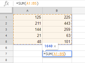
Google Sheets uses not only single cell references but also groups of adjacent cells – ranges. They are limited by the upper left and bottom right cells. For instance, A1:B5 signals to use all cells highlighted in orange below:
Constants in Google Sheets formulas
Constant values in Google Sheets are the ones that cannot be calculated and always remain the same. Most often, they are numbers and text, for example 250 (number), 03/08/2019 (date), Profit (text). These are all constants and we can alter them using various operators and functions.
For example, the formula may contain only constant values and operators:
=30+5*3
Or it can be used to calculate new value based on another cell's data:
=A2+500
Sometimes, though, you have to change the constants manually. And the easiest way to do that is to place each value into a separate cell and reference them in formulas. Then, all you need to do is make changes in a single cell rather than in all formulas.
So, if you put 500 to B2, refer to it with the formula:
=A2+B2
To get 700 instead, simply change the number in B2 and the result will be recalculated.
Operators for Google Sheets formulas
Different operators are used in spreadsheets to preset the type and the order of calculations. They fall into 4 groups:
- arithmetic operators
- comparison operators
- concatenation operators
- reference operators
Arithmetic operators
As the name suggests, these are used to perform math calculations such as adding, subtracting, multiplication, and division. As a result, we get numbers.
| Arithmetic operator | Operation | Example |
| + (plus sign) | Addition | =5+5 |
| - (minus sign) | Subtraction Negative number |
=5-5 =-5 |
| * (asterisk) | Multiplication | =5*5 |
| / (slash) | Division | =5/5 |
| % (percent sign) | Percents | 50% |
| ^ (caret sign) | Exponents | =5^2 |
Comparison operators
Comparison operators are used to compare two values and return a logical expression: TRUE or FALSE.
| Comparison operator | Comparison condition | Formula example |
| = | Equal to | =A1=B1 |
| > | More than | =A1>B1 |
| < | Less than | =A1<B1 |
| >= | More than or equal to | =A1>=B1 |
| <= | Less than or equal to | =A1<=B1 |
| <> | Not equal to | =A1<>B1 |
Text concatenation operators
Ampersand (&) is used to connect (concatenate) multiple text strings into one. Enter the below into one of Google Sheets cells and it will return Aircraft:
="Air"&"craft"
Or, put Surname to A1 and Name to B1 and get the Surname, Name text with the following:
=A1&", "&B1
Formula operators
These operators are used to build Google Sheets formulas and indicate data ranges:
| Formula operator | Action | Formula example |
| : (colon) | Range operator. Creates reference to all cells between (and including) the first and the last cells mentioned. | B5:B15 |
| , (comma) | Union operator. Joins multiple references into one. | =SUM(B5:B15,D5:D15) |
All operators are of different priority (precedence) that defines the order of formula calculations and, most often, affects the resulting values.
Order of calculations and operators precedence
Each formula in Google Sheets handles its values in some particular order: from left to right based on operator precedence. Operators of the same priority, e.g. multiplication and division, are calculated in the order of their appearance (left to right).
| Operators precedence | Description |
| : (colon) (space) , (comma) |
Range operator |
| - | Minus sign |
| % | Percentage |
| ^ | Exponentiation |
| * and / | Multiplication and division |
| + and - | Addition and subtraction |
| & | Concatenate multiple textual strings into one |
| = <> <= >= |
Comparison |
How to use brackets to change the order of calculations
To change the order of calculations within the formula, enclose the part that should come first into brackets. Let's see how it works.
Suppose we have a standard formula:
=5+4*3
Since multiplication takes the lead and addition follows, the formula will return 17.
If we add brackets, the game changes:
=(5+4)*3
The formula adds numbers first, then multiplies them by 3, and returns 27.
The brackets from the next example dictate the following:
=(A2+25)/SUM(D2:D4)
- calculate value for A2 and add it to 25
- find the sum of values from D2, D3, and D4
- divide the first number to the sum of values
I hope it won't be difficult for you to get around these since we learn the order of calculations from a very young age and all arithmetics around us are performed this way. :)
Named ranges in Google Sheets
Did you know you can label separate cells and entire data ranges? This makes processing large datasets quick and easy. Besides, you will guide yourself within Google Sheets formulas much faster.
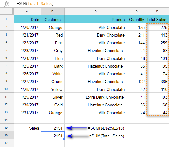
Suppose you have a column where you calculate total sales per product and customer. Name such a range Total_Sales and use it in formulas.
I believe you would agree that the formula
=SUM(Total_Sales)
is far clearer and easier-to-read than
=SUM($E$2:$E$13)
Note. You can't create named ranges from non-adjacent cells.
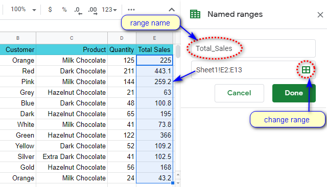
To identify your range, do the following:
- Highlight your adjacent cells.
- Go to Data > Named ranges in the sheet menu. A corresponding pane will appear on the right.
- Set the name for the range and click Done.
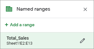
Tip. This also lets you check, edit, and delete all ranges you've created:
Picking correct name for the data range
Named ranges make your Google Sheets formulas friendlier, clearer, and understandable. But there's a small set of rules you should follow when it comes to labeling ranges. The name:
- Can contain only letters, numbers, underscores (_).
- Should not start from a number or from "true" or "false" words.
- Should not contain spaces ( ) or other punctuation marks.
- Should be 1-250 characters long.
- Should not tally with the range itself. If you try to name the range as A1:B2, the errors may occur.
If something goes wrong, e.g. you use space in the name Total Sales, you'll get an error right away. The correct name would be TotalSales or Total_Sales.
Note. Google Sheets named ranges are similar to absolute cell references. If you add rows and columns to the table, the Total_Sales range won't change. Move the range to any place of the sheet – and this won't alter the results.
Types of Google Sheets formulas
Formulas can be simple and complex.
Simple formulas contain constants, references to cells on the same sheet, and operators. As a rule, it's either one function or an operator, and the order of calculations is very simple and straightforward – from left to right:
=SUM(A1:A10)
=A1+B1
As soon as additional functions and operators appear, or the order of calculations becomes a bit more complicated, the formula becomes complex.
Complex formulas may include cell references, multiple functions, constants, operators, and named ranges. Their length can be overwhelming. Only their author can "decipher" them quickly (but usually only if it was built not more than a week ago).
How to read complex formulas with ease
There is a trick to make your formulas look comprehensible.
You can use as many spaces and line breaks as you need. This won't mess with the result and will arrange everything in the most convenient way.
To put a break line in the formula, press Alt+Enter on your keyboard. To see the entire formula, expand the Formula bar:
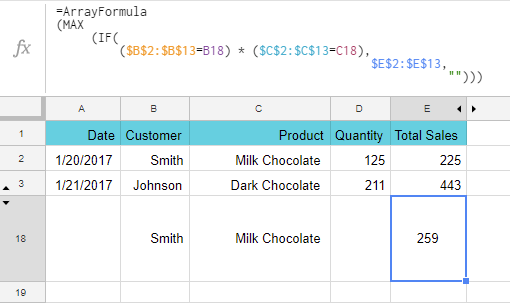
Without these extra spaces and break lines, the formula would look like this:
=ArrayFormula(MAX(IF(($B$2:$B$13=B18)*($C$2:$C$13=C18), $E$2:$E$13,"")))
Can you agree the first way is better?
Next time I'll dig deeper into building and editing Google Sheets formulas, and we'll practice a bit more. If you have any questions, please leave them in the comments below.
 by
by
43 comments
Hello,
I am new to sheets and data and am wanting a formula/function to give numerical value to another number based on the position in a race (ie, 1, 2, 3, 4 etc) to give those positions a value of points.
So 1 = 10 points, 2 = 9 points etc where I can place the race order in once column beside a name and then have the points value automatically calculated.
Thanks
Hello Garth,
If I understand your task correctly, you can either:
Hi
i want to know how number value is converted into words in excel
Hi! The answer to your question can be found in this article: How to convert number to words in Excel.
I am BEW to google sheets and similar type of programs and I am using an IF statement to know the content of a cell in google sheets so I can know the content of 2 cells and substract one from another. I am using Row() to know the cell number example: I((Row())+1) - I(Row()). It's about "Difference Previous" like context so the lower cell minus the higher cell but I don't know the cell number so I want to know based on an IF Clause if the cell I am checking is lower then the "following cell minus current cell" let's say column I, I want to know the location of the cell so I used Row() but when combined "I(ROW())+1 - I(ROW())" I am getting an error. Can you help me here ???...
Thank you.
Hello Fady,
Sorry, what do those I symbols before each Row() mean? Have you tried using the IF formula? We have a detailed tutorial about it.
Is there a character that can be used to disable portions of a formula? For example, I want to use the FILTER formula to combine information from multiple sheets (I am a teacher and want to combine multiple class rosters into a single combined "all-class" roster). To save time, I would prefer to have a comprehensive formula containing FILTER functions for all possible classes that I COULD teach, but disable any individual FILTER functions for classes/courses I am not teaching during a specific year.
Here is the "comprehensive" formula I would like to use:
={FILTER('APB 1'!B2:D,'APB 1'!D2:D"");FILTER('APB 2'!B2:D,'APB 2'!D2:D"");FILTER('APB 3'!B2:D,'APB 3'!D2:D"");FILTER('APB 4'!B2:D,'APB 4'!D2:D"");FILTER('APB 4'!B2:D,'APB 4'!D2:D"")}
For this formula to work I have to have data on the following sheets: APB 1, APB 2, APB 3, APB 4, and APB 5. BUT if I am only teaching some but not all of these classes is it possible to disable individual FILTER functions so that the spreadsheet will ignore them? I tried surrounding them with "s, 's, [s, and |s. but none of them worked.
Thanks in advance for any help you can provide!
Stefan
Hello Stefan,
If I understand your task correctly, the sheets APB 1-5 will remain empty if you don't teach the classes. In cases like this, you can try incorporating the IF function that will check if the data is there in some column and take it into the filter only if it is.
Alternatively, try using the QUERY function. It has no problems skipping the data if it's not there on the sheets.
Natalia, thank you very much! I used the Query function and it worked!
Thank you for the update, Stefan, glad I could help! :)
Hi Team
I will try my best to describe my requirements.
Background:
I would like to reproduce the Table of Contents which is in my Google Docs in a Google sheet. Now as this can change over time I want to copy it into a tab "raw data". I would like to create another tab to just copy the data across from the raw data tab. As the copy and paste is only produced in one column the requirement is two fold:
1. To show the data over 3 columns: Heading / Sub Heading / Sub-Sub Heading just as it is presented in the Table of Contents
2. To combine the 3 columns without numbering in front and with a sign of > in-between the 3 columns data
Example:
Row 1 = Headings of Columns
Row 2 = 9.0 Research Tools
Row 3 = 9.1 Quick Compare
Row 4 = Insurance Review
The result required for 1st requirement:
Cell B2 = 9.0 Research Tools ( so every number with #.0 should be in Column B)
Cell C3 = 9.1 Quick Compare ( so every number > than with #.0 should be in Column c)
Cell D4 = Insurance Review ( so everything without a number should be in Column D)
The result required for 2nd requirement:
Cell E3 = Research Tools > Quick Compare
Cell E4 = Research Tools > Quick Compare > Insurance Review
I'm looking forward to your response.
Kind regards,
Hi Etienne,
If I understand your task correctly, I'd advise trying the following:
Thanks Natalia for your reply,
Re: Vlookup formula - I'm unsure how to use this if there is no table to return something from?
Sorry I was not clear on the example information. The raw data is in column A.
A1 = Headings of Columns
A2 = 9.0 Research Tools
A3 = 9.1 Quick Compare
A4 = Insurance Review
The formula in Columns B, C, D should have the following result:
Cell B2 = 9.0 Research Tools ( so every number with #.0 should be in Column B)
Cell C3 = 9.1 Quick Compare ( so every number > than with #.0 should be in Column c)
Cell D4 = Insurance Review ( so everything without a number should be in Column D)
I'll have a look at the how guides you have provided the links for for requirement 2
Thank you for the clarifications, Etienne.
Below are the formulas you can use. I created them in a way so they look at all cells in the A1:A10 range in one go. Change A10 depending on how many rows you have.
For column B:
=ArrayFormula(IFERROR(IF(SEARCH(".0",$A$1:$A$10,1)>0,$A$1:$A$10,""),""))
For column C:
=ArrayFormula(IFNA(IF((REGEXEXTRACT($A$1:$A$10,"\.(\d+)")+0)>0,$A$1:$A$10,""),""))
For column D:
=ArrayFormula(IF(ISNA(REGEXEXTRACT($A$1:$A$10,"\.(\d+)")=TRUE),$A$1:$A$10,""))
Feel free to learn more about ArrayFormula, IF function and REGEXEXTRACT on our blog.
Natalia, you're a champion. I'm not sure what these formulas are all about, but it works perfectly. Thank you so much. I like the arrayformula at the start which helps when we have to manually insert or delete a row. The only issue I have now is that I get "ref" issues in other tabs referencing data in this tab. This happens even when I use the function arrayformula. This is only when I delete a row. Is there a way to allow for deleting of rows and inserting rows in the source tab which will not influence any formulas in other tabs?
Is it possible to use a pivot table to see exactly the way the data will display for Column's B,C & D. In this way I can use formulas in column E and so on which will never have ref issues.
Again, thank you for your help!
Hi Natalia
In reference to the above I hope my issue will be solved if all the columns to the right of Column B,C&D also has the Arrayformula. However I have some difficulty as some has a Circular dependency detected.
Based on the results of your formulas , what I'm trying to get as a result in Column E:
Column E/Cell B2 = Research Tools
Column E/Cell C3 = Research Tools > Quick Compare
Column E/Cell D4 = Research Tools > Quick Compare > Insurance Review
The current formulas I'm using:
Column E (works only if the other columns it reference has no issues):
=ARRAYFORMULA(F4:F200&IF(G4:G200="",""," > "&G4:G200)&IF(H4:H200="",""," > "&H4:H200))
Column F (which has a Circular dependency issue):
=arrayformula(IF(B4:B200"",MID(B4:B200,FIND(" ",B4:B200)+1,LEN(B4:B200)),IF(F3:F200="","",F3:F200)))
Column G (which has a Circular dependency issue):
=arrayformula(iF(B4:B200"","",IF(C4:C200="",G3:G200,MID(C4:C200,FIND(" ",C4:C200)+1,LEN(C4:C200)))))
Column H (which works fine):
=ARRAYFORMULA(IF(B4:B200"","",IF(C4:C200"","",D4:D200)))
Any idea how to combat this as well
Thank you
Hi Etienne,
Would it be possible for you to share an editable copy of your spreadsheet with formulas with me: support@apps4gs.com?
I'll see why circular dependency occurs directly in your file and try to help.
Note. We keep that Google account for file sharing only and don't monitor its Inbox. Please do not email there. Once you share the file, just confirm by replying to this comment.
I have =sum(b20:x20) if I color in a box say green, can it take away from the sum
Hello Josh,
I'm sorry, your task is not clear. If you still need help with it, please describe it in detail.
A Google Sheet code is as follows:-
=If(B2 " ", GOOGLEFINANCE(B2, "NAME"), " ")
=If(B2 " ", What is the meaning of this symbol " " after
GOOGLEFINANCE(B2, "NAME"), " ") What is the meaning of this symbol " " at the end of the code
Would be very thankful for an answer.
Hi George,
It tells IF to keep the cell empty if the condition is not met. You can learn more about the IF function in this blog post.
Are you able to get the intersect operator to work in Sheets? I can in Excel but not Google Sheets. I get a formula parse error.
Hi Adam,
Indeed, at the moment it doesn't work the same way as in Excel and as described in this blog post. I'll delete this operator from the article as an obsolete one. Thanks for the catch!
I am seeking a reference for all syntactic operators in sheets. This is close but misses brace (curly bracket), semicolon and comma as used in array syntax.
Hello Pete,
This guide covers the very basics while the array formulas are the next level.
The array syntax is explained whenever it's used in the related blog posts. Like this one, for example.
Holy cow. I'm self-learning how to do formulas and queries and such in Google Sheets (and Excel when I get the opportunity) and I've been looking for a week for a list that had these symbols (or operators and I'm probably still calling it the wrong thing) and what they mean. Very helpful. Thank you.
I'm trying to see if there is a formula for adding A1 and B1 and A2 and B2 simply using the same formula for both equations? Can it be replicated for all A values and B values?
Hello Isaac,
I'm sorry but your task is not clear. For me to be able to suggest anything, please describe what you're trying to do in detail. Thank you.
I am creating a spreadsheet for my cattle operation(which is small) I have cattle listed by tag color and number on tag. Is there a formula that I can apply to the spreadsheet that when I put in information in the form concerning a specific color for the ear tag and then a specific # value of the ear tag,It will populate in my spreadsheet in the proper corresponding cell range for that Cow I have listed for the color and # in my spreadsheet in sequence, without creating random entries at the bottom of the spreadsheet?
Hello Randall,
If I understand your task correctly, you could try using VLOOKUP or INDEX MATCH functions to pull responses returned by your form to whenever you need.
=SUM(SUMIFS(AH11,H11,{"W","R","F","G"}))
In excel the above formula returns a value if WRF or G is found in H11
In google sheets it only returns a value for the first item, in this case "W"
How do I get sheets to return a value if any of the four letters are found in H11?
Hello Arch,
The following article explains the SUMIFS function in Google Sheets:
Sum cells with multiple OR criteria
I have multiple identical sheets with different values within a database. I want to create a summary sheet that would pull one line of data from each of the other sheets where the date field equals today. Any help with the formula?
Hi Mike,
If you want to use standard formulas, I'd suggest you have a look at Google Sheets QUERY and IMPORTRANGE. INDEX MATCH is also capable of pulling entire rows based on the condition.
However, there's a much simpler way - we have a special add-on, Multiple VLOOKUP Matches, for the task. You can test it out for 30 days for free. These instructions will help you get to know the tool better.
I am working on a calculation that try's to create a number for say in cell D1, that takes a value input in say A1 subtracts a value in cell C1 from it, if the result if less than 0 , or minus ( ) , it reports 0, but if the number has a positive value , it then multiply's that number by cell E1 which is a percentage . For example
EXAMPLE 1 - A1 = 100 MINUS B1= 50 = D1 which would report 50 then X 11.5% would equal 5.75
HOWEVER EXAMPLE 2 A1 = 100 MINUS B1= 150 = D1 which would report (50) then X 11.5% would equal 0 . I THINK THIS IS A "IF" KIND OF CALCULATION, Any hints would be most welcome
Hello Andrew,
You're absolutely right, it's the IF function that is used to solve such tasks. You should be able to create the formula by following examples from this blog post: IF function in Google Sheets
Hi there,
I'm relatively simple as far as spreadsheets go but have been battling with something that I am not sure can be achieved, here goes...
I have a simple finance spreadsheet that I use at home and I want to create a calculation that will be relative to a column that I delete each month, so it is replaced with the current month (there are 12 months in total).
Each time I delete the current column, I receive the #REF error in the calculation of the field that contains my calculation, seemingly because I have deleted the previous column. What I'm trying to do is fix the calculation so that it is clever enough to read the 'new ' column that has replaced the deleted one.
I have message around with different formulas but nothing seems to work, help!
Hi Phill,
I believe our Advanced Find and Replace will help you. By looking in formulas, it will find all references to the deleted column and change them all at once to the new reference. You can test the add-on for 30 days for free to see if it works as desired.
Is it possible to count 1,2,3 in a single cell as 6. Say cell A1 has 123 in it and you want to add the numbers together in cell cell A2 to =6
Yes, it is, Colin. Try this:
=SUMPRODUCT(1*MID(A1,ROW(INDIRECT("1:"&LEN(A1))),1))
So I have a google sheet with multiple formulae in it. When I duplicate the sheet, the formuale don't work anymore. Help?
Hello Shane,
There are plenty of reasons for that, I'm afraid.
Perhaps, the references take too long to update, especially if there are too many formulas. It can be your internet connection speed/quality or a not-so-powerfull computer. You could also try and check the settings of the spreadsheet and its locale.
thanks..that was super helpful...I have been trying to figure out absolute values for ever without knowing what I was looking for. It really clarified how sheets works..Cannot thank you enough!!
cheers
Amy