If you only know how to make a basic filter in Google Sheets, I have a surprise for you! Come, we'll discover the Google Sheets FILTER function together. You will find many ready-made formulas and one powerful tool that complements the filtering toolset immensely.
Some time ago we explained how to filter data in Google Sheets using the standard tool. We mentioned how to filter by value, by condition & by color using standard Google Sheets tools. However, spreadsheets always have more in them than we know. And this time I'm going to introduce you to the Google Sheets FILTER function.
Syntax of the Google Sheets FILTER function
FILTER function in Google Sheets scans your data and returns the required information that meets your criteria.
Unlike the standard Google Sheets filter, the function doesn't do anything with your original data. It copies the found rows and puts them wherever you build the formula.
The syntax is pretty easy since each argument speaks for itself:
- range is the data set you want to filter. Required.
- condition1 is a column or row along with the TRUE/FALSE criteria it should fall under. Required.
- condition2,..., etc., stand for other columns/rows and/or their criteria. Optional.
Note. Each condition should be of the same size as the range.
Note. If you filter by multiple conditions, they should all be either for columns or rows. Google Sheets FILTER function doesn't allow mixed conditions.
Now, with these notes in mind, let's see how how these arguments shape different formulas.
How to use FILTER function in Google Sheets with text
I'm going to show you all examples by filtering a small table with some orders:
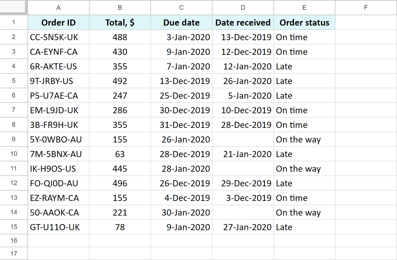
There are different types of data in this table and only 15 rows which is perfect to learn the FILTER function.
Example 1. Text is exactly
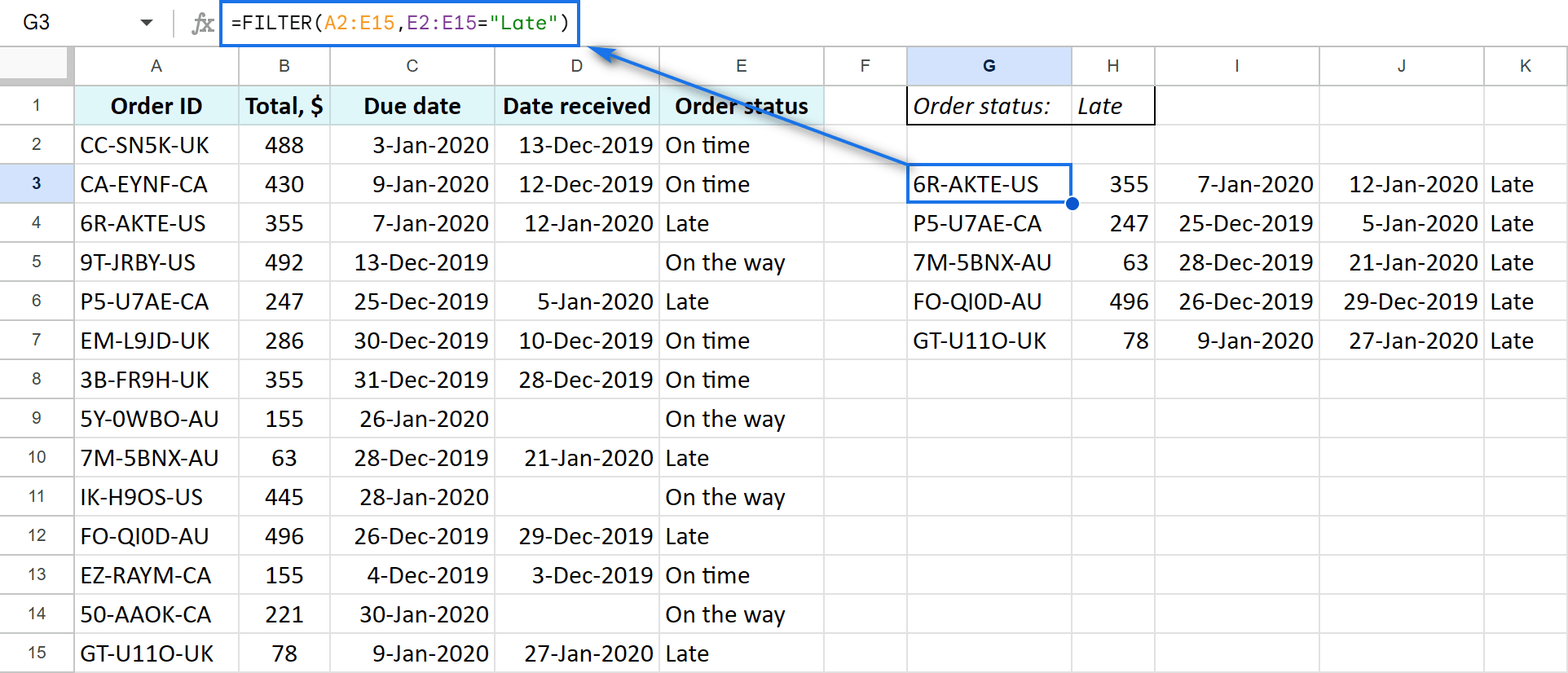
First, let's ask the function to get only those orders that are running late. Their status is saying exactly Late. I enter the range I want to filter — A2:E15 — and then set the condition — column E should equal Late:
=FILTER(A2:E15,E2:E15="Late")
Example 2. Text is exactly not
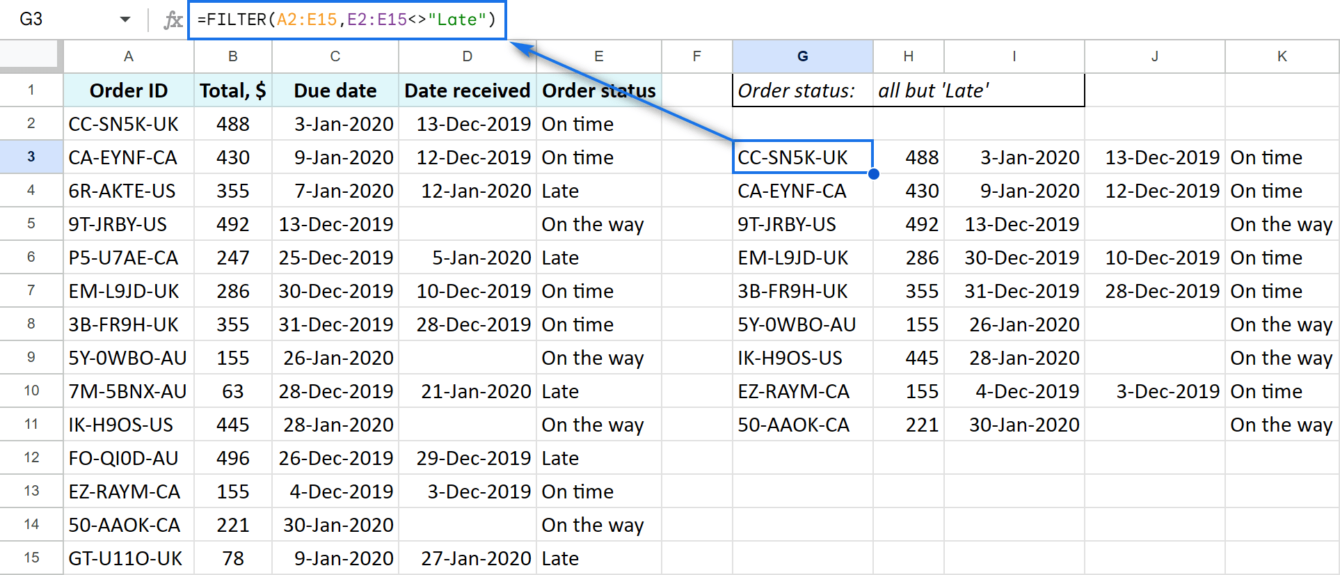
Now let's do the opposite: get all orders but those that are late. For that, you will need a special comparison operator (<>) that means not equal to. Google Sheets FILTER function will return all rows where the contents of column E is opposite to a word Late:
=FILTER(A2:E15,E2:E15<>"Late")
Google Sheets FILTER formula contains text: partial matches, case-sensitive filter
Now let's filter this Google Sheets data by partial matches. I'll look for all cells where text contains just the needed part. It doesn't have to be the only contents of cells — only a part will be enough.
Normally, you'd use wildcard characters for this task. But when building Google Sheets FILTER formulas, it is FIND and SEARCH functions that operate this way.
And it further depends on whether your search is case-sensitive. If so, pick FIND. Otherwise, opt for SEARCH.
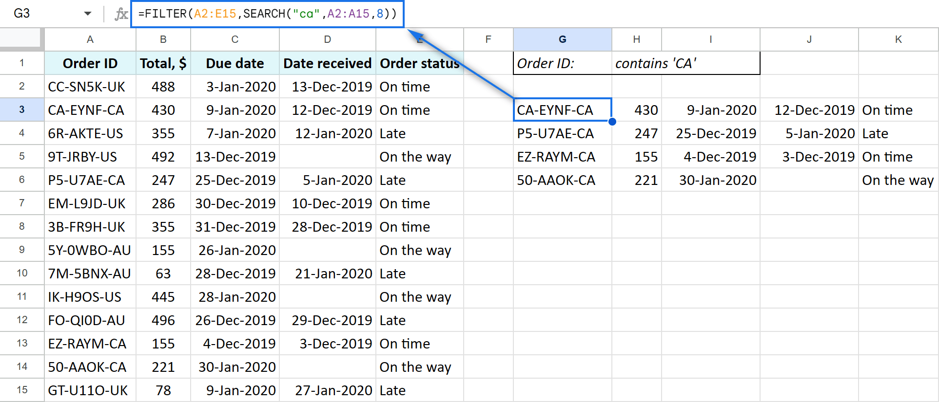
Did you notice that order IDs in column A mention countries at their end? This next formula will filter only orders shipped from Canada (CA).
The SEARCH function will do just fine for my example since the text case is irrelevant:
- search_for is the text you want to find. You must wrap it in double-quotes: "ca". Required.
- text_to_search is the range to scan for the needed text: A2:A15. Required.
- starting_at indicates the starting position for the search — the number of the character to start looking from. It's completely optional but I need to use it. You see, all order IDs consist of letters and numbers, meaning a pair of CA may occur somewhere in between as well. Yet. the identical pattern of all IDs lets me look for CA starting from the 8th character.
After collecting all these parts together, your Google Sheets filter formula will look like this:
=FILTER(A2:E15,SEARCH("ca",A2:A15,8))
How to filter in Google Sheets using cell references
Each time you create a Google Sheets filter formula, you need to enter the condition as is: whether a word or its part, the date, etc. Unless you're familiar with cell references.
They make lots of things about formulas easier. Because instead of typing everything out, you can simply refer to cells with conditions.
Remember how I looked for all late orders? I can quickly refer to E4 with the text Late to do the same:
=FILTER(A2:E15,E2:E15=E4)
The result won't differ at all:
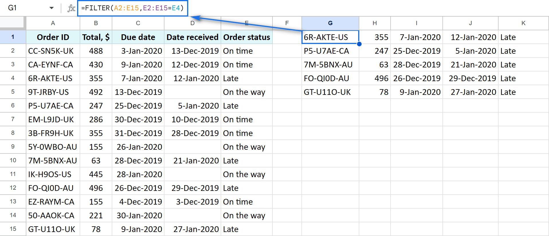
You can repeat this with all the formulas. For example, avoid adding more functions like DATE and just refer to the cell with a date of interest:
=FILTER(A2:E15,C2:C15=C15)
Tip. Cell references also let you filter from another Google sheet. You just have to bring the sheet name:
=FILTER(Orders!A2:E15,Orders!C2:C15=Orders!C15)
Google Sheets FILTER function with date and time
To use the Google Sheets FILTER function with date and time, you will need additional functions. Based on your task, you may need to embed DAY, MONTH, YEAR, DATE and TIME.
Tip. If you're not familiar with these functions or simply find them tricky and don't want to mess things up with dates, look at the tool described at the end. It doesn't require any functions at all!
Example 1. Date is
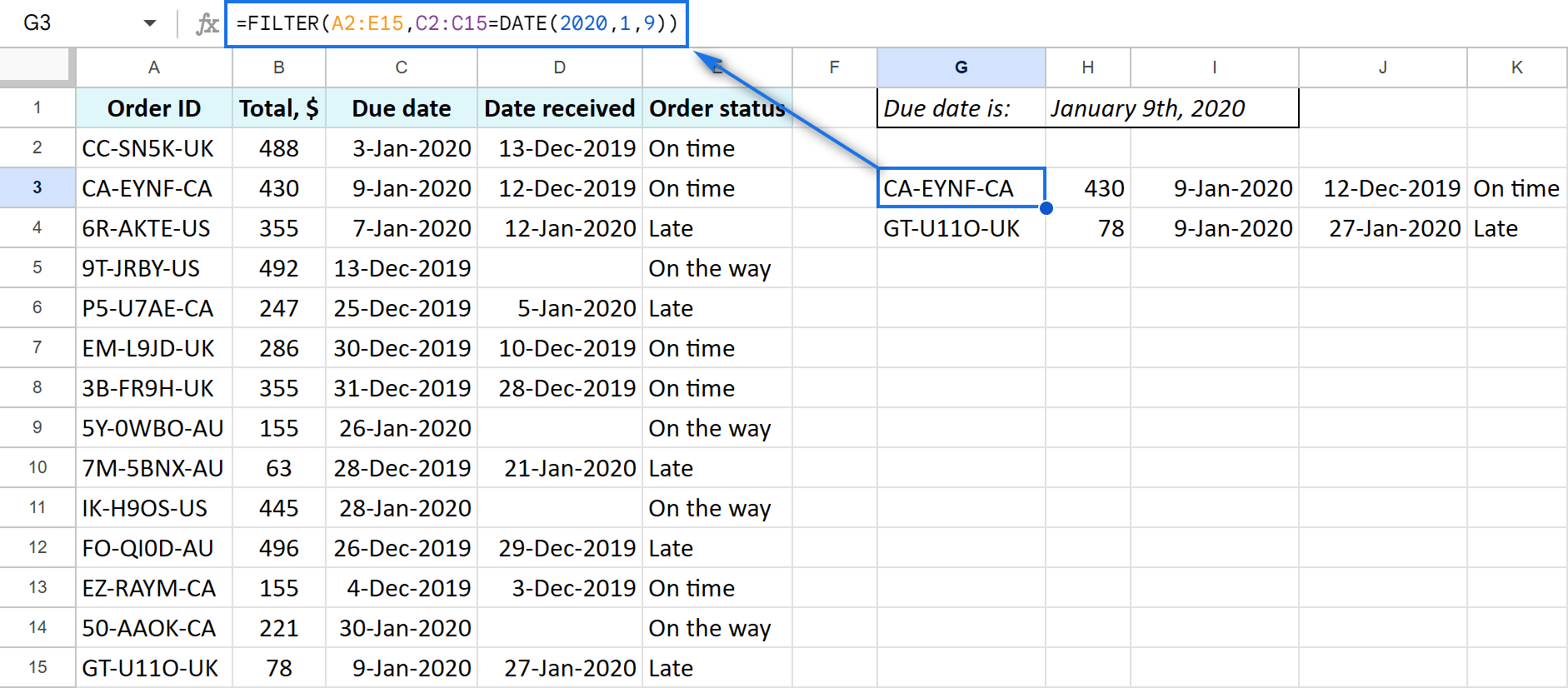
Let's find orders that should arrive on January 9, 2020. To use FILTER function in Google Sheets with date, you will need the DATE function:
=FILTER(A2:E15,C2:C15=DATE(2020,1,9))
Example 2. Date contains
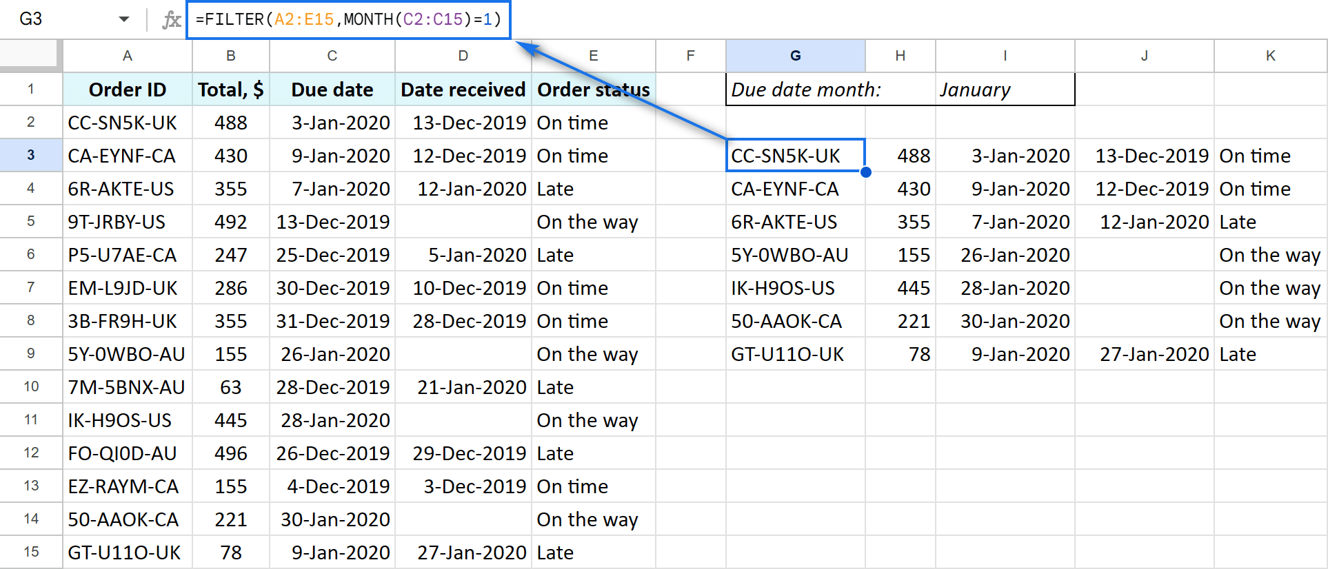
If you're interested in a particular month or a year only, you can get by with MONTH and YEAR functions. Put the range with dates (C2:C15) right into the functions and specify the number of the required month (or year). In my case, it's January so it's 1 (=1):
=FILTER(A2:E15,MONTH(C2:C15)=1)
Example 3. Date is before/after
To extract data that falls before or after certain dates, you will need the DATE function and such comparison operators as greater than (>), greater than or equal to (>=), less than (<), less than or equal to (<=).
Here is the formula for orders that arrived on and after January 1, 2020:
=FILTER(A2:E15,D2:D15>=DATE(2020,1,1))
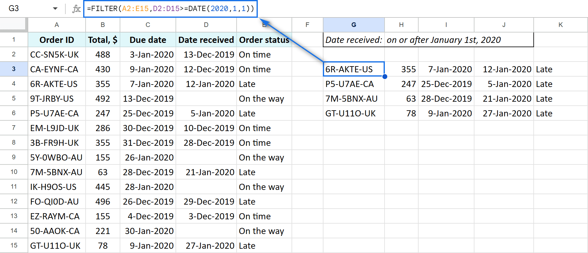
Of course, you can also use MONTH or YEAR here. The result will be the same:
=FILTER(A2:E15,YEAR(D2:D15)>=2020)
Example 4. Time
When filtering Google Sheets by time, the drill is the same as with dates. Only this time, you use the TIME function:
For instance, to get only records with a timestamp after 2:00 PM, the FILTER formula will be:
=FILTER(A2:B10,A2:A10>TIME(14,0,0))
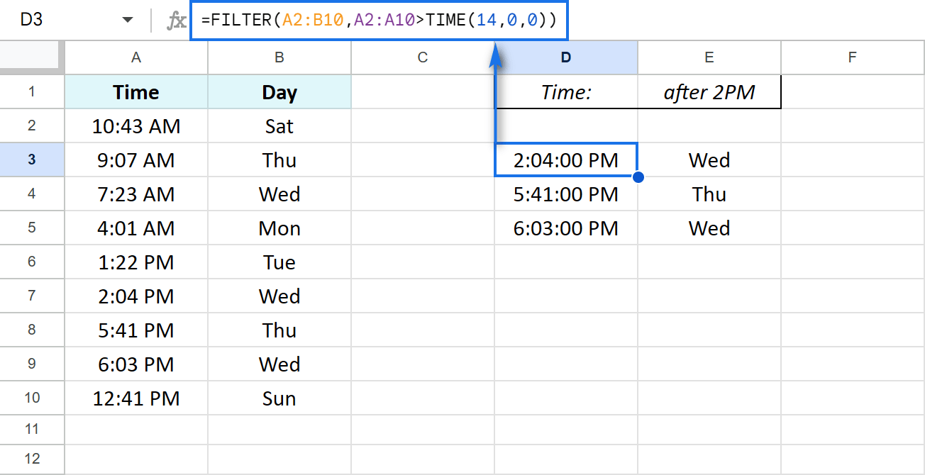
You may think you could use the HOUR function just like MONTH for dates to specify certain hours. But the game changes a bit here. Time in Google Sheets is tricky enough meaning a few adjustments will be necessary.
To extract all rows where time is between 2:00 PM and 12:00 PM, do this:
- Wrap the range with timestamps (A2:A10) in a separate HOUR function. This will signal where to look.
- Then add another HOUR function to set the time itself.
=FILTER(A2:B10,HOUR(A2:A10)>=HOUR("2:00:00 PM"))
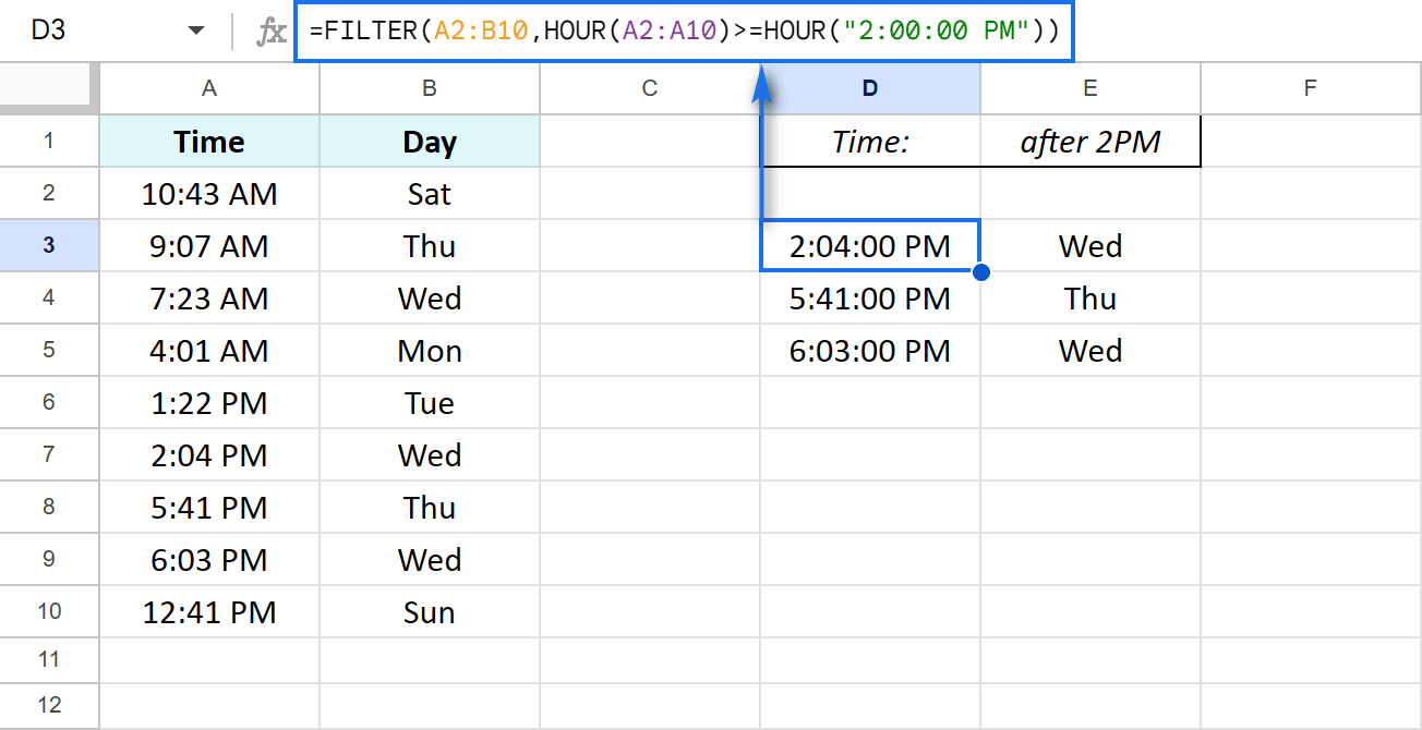
Tip. See that the result doesn't include 12:41 PM? That's because the spreadsheet treats it as 00:41 which is less than 2:00.
If you find a more elegant solution, please share it in the comments section below.
Filter by color: custom formula for Google Sheets
Chances are, you're no stranger to using colors to organize your spreadsheet data better. But did you know that Google Sheets FILTER function can process colors too? There's just one catch — it needs help from another custom function: CELLCOLOR.
This function comes bundled with our Function by Color add-on for Google Sheets. You can install it and try for free right now to see firsthand how the FILTER and CELLCOLOR combo works.
Let me show you how it works. There are some orders I expect most and least. I'll color them light purple and light yellow respectively:
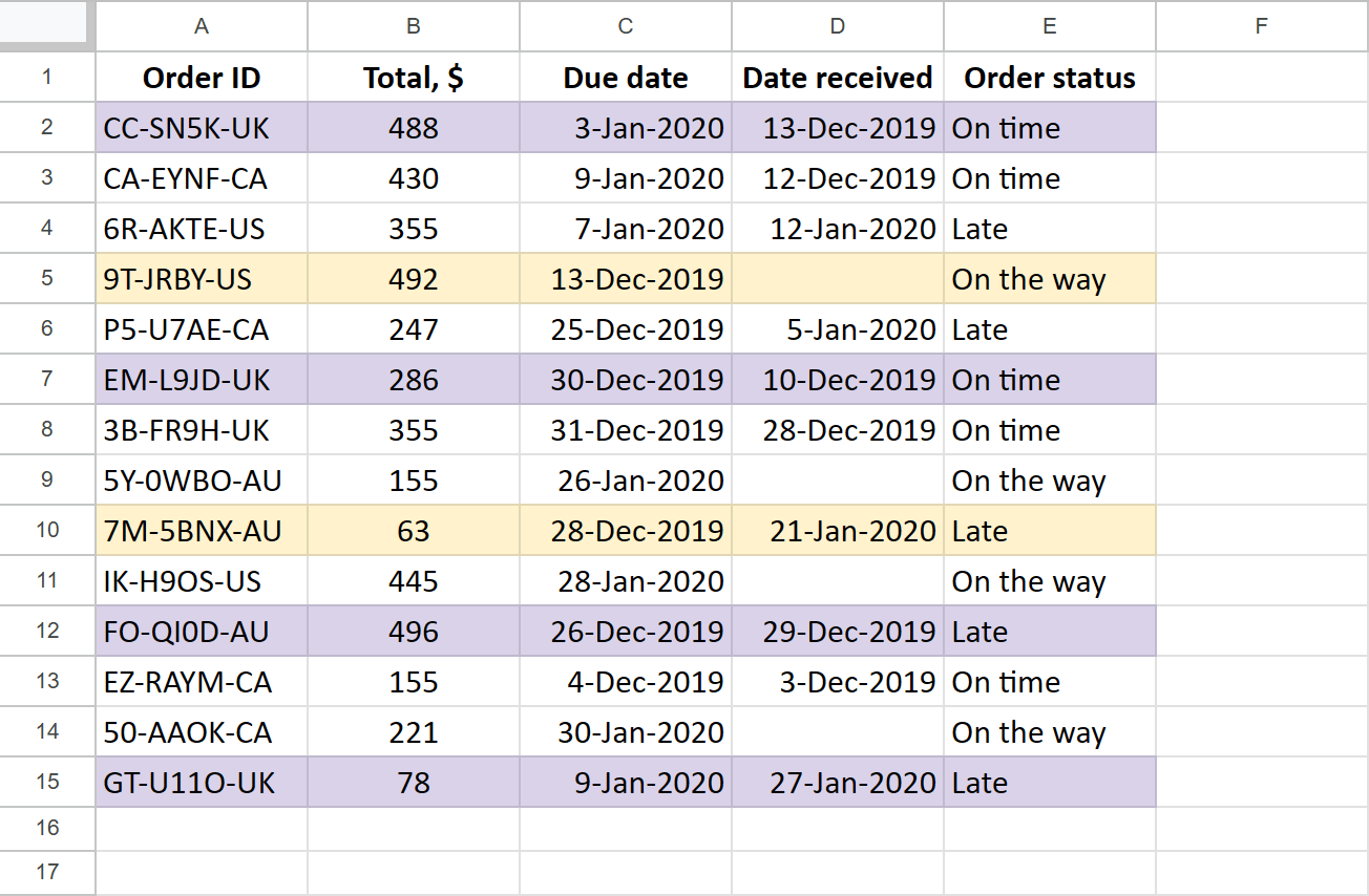
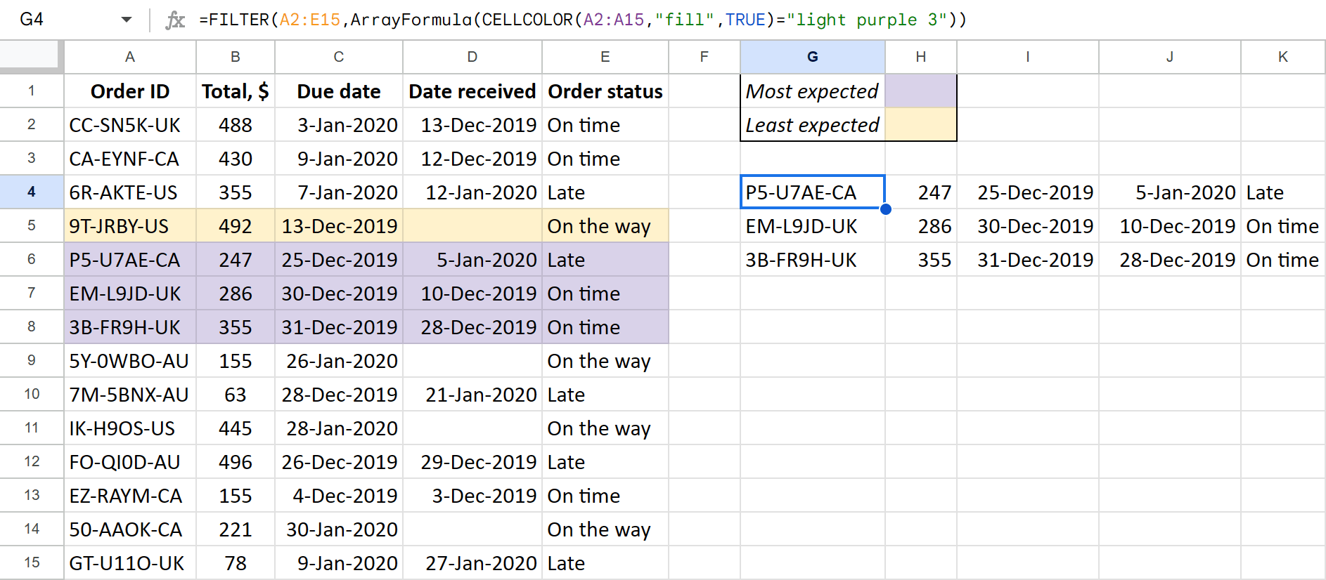
I'm going to filter this table by color to show only most expected orders (the purple ones). For that, I will use Google Sheets FILTER function with the CELLCOLOR function embedded:
=FILTER(A2:E15,ArrayFormula(CELLCOLOR(A2:A15,"fill",TRUE)="light purple 3"))
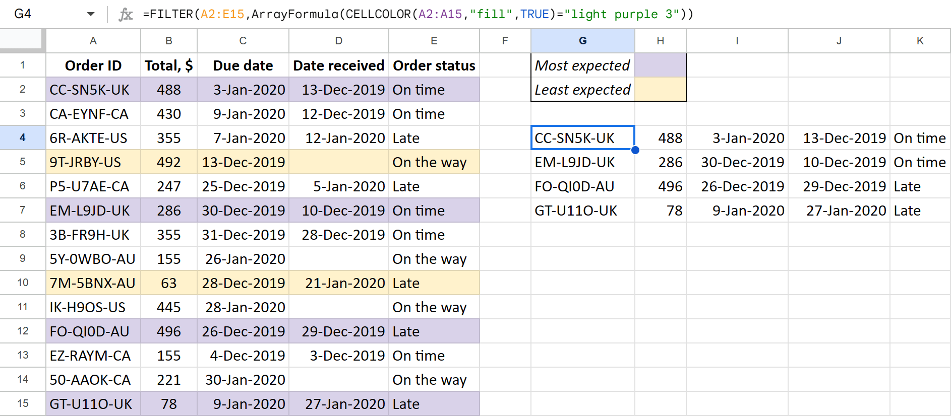
Here's how the formula works exactly:
- CELLCOLOR looks through each cell in A2:A15.
- Takes their fill colors.
- And uses ArrayFormula to pass the list of color names to the FILTER function.
- FILTER function then scans the whole table: A2:E15.
- And extracts only those rows where the fill color is "light purple 3" according to CELLCOLOR list.
There are 4 such rows in my table and these functions do a perfect job of filtering and extracting them.
How to refresh your filter if colors change
There's one thing to remember when working with colors in Google Sheets. If you recolor your original data set, the formula result won't update automatically because color changes in spreadsheets don't trigger formula updates:

By default, this happens in spreadsheets only when you change values.
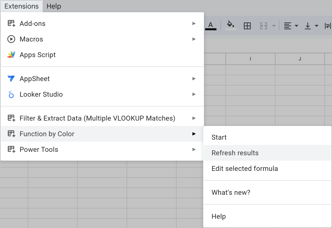
But CELLCOLOR comes prepared. It's a part of the Function by Color add-on for this exact reason — to spare you the trouble of messing with records. So to update the result if only colors change, simply select Extensions > Function by Color > Refresh results:
Once you initiate this refresh, the formula will filter your table by color once again extracting the updated result:
Google Sheets FILTER function for multiple criteria
While I mainly used one condition in all Google Sheets filter formulas before, it is more likely that you'll need to filter your Google Sheets by multiple criteria at once. Here are a few examples.
Google Sheets FILTER + AND function
So how do you filter by multiple criteria in one column? To find all rows falling between two numbers/dates/times, the optional arguments of the FILTER function — condition2, condition3, etc. — will come in handy. You just duplicate the same range each time but with a new condition.
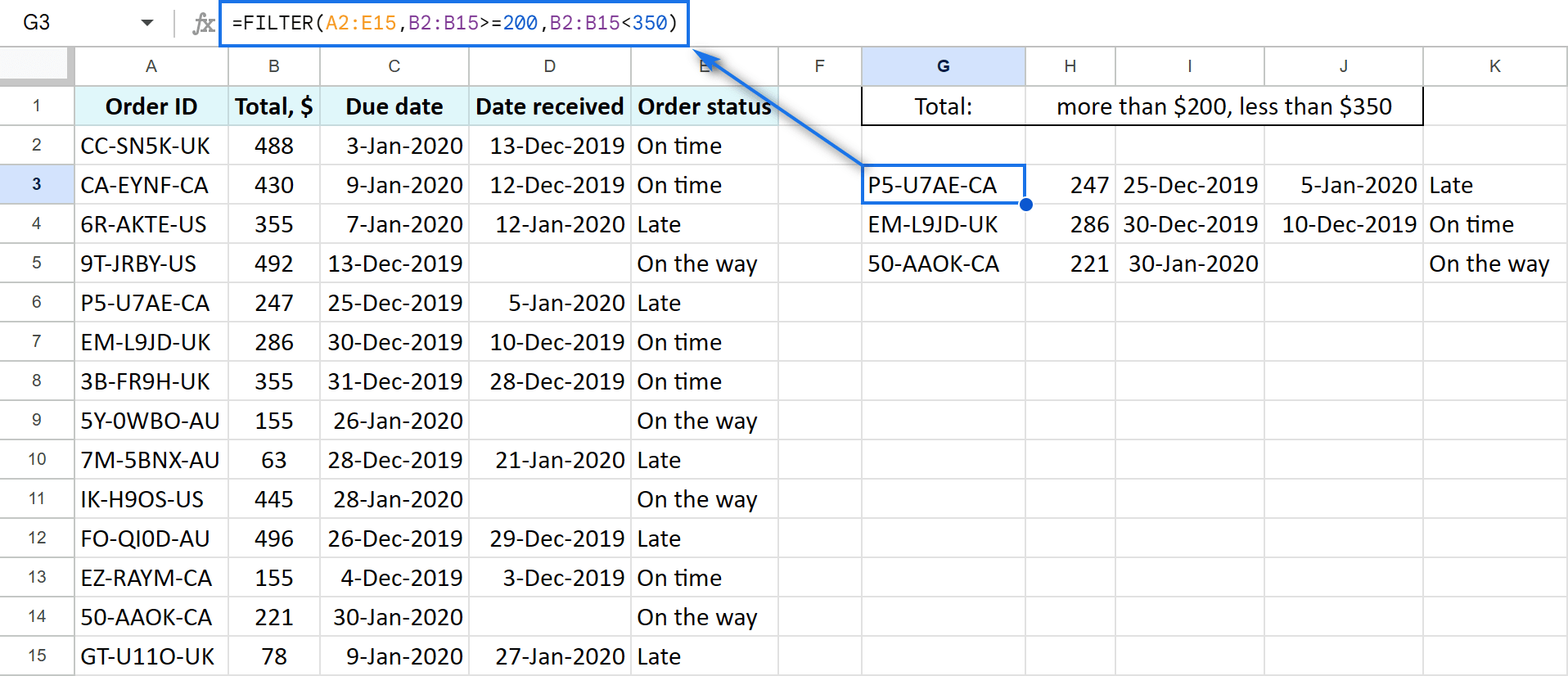
Check this out, I'm going to return only those orders that cost me more than $200 but less than $350:
=FILTER(A2:E15,B2:B15>=200,B2:B15<350)
Google Sheets FILTER function — OR condition
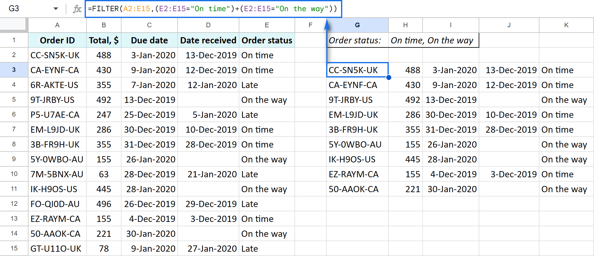
Will the same work to extract rows that contain either this or that record within one column (OR condition)? For instance, how do you check all orders that are both on their way and late?
To correctly set up the Google Sheets FILTER function for the OR condition, you should sum these two criteria within one argument:
=FILTER(A2:E15,(E2:E15="On time")+(E2:E15="On the way"))
Google Sheets FILTER function for multiple columns
What's even more likely than applying a few conditions to one column is creating a filter in Google Sheets for multiple columns.
The arguments are all the same. But each new part of the formula requires a new range with its own criteria.
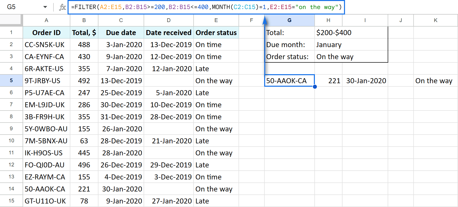
Let's try and make the FILTER function in Google Sheets extract orders that fall under all the following rules:
- They should be $200-400 worth:
A2:E15,B2:B15>=200,B2:B15<=400 - Arriving in January 2020:
MONTH(C2:C15)=1 - But are still on their way:
E2:E15="on the way"
Put all these parts together and your Google Sheets filter formula for multiple columns is ready:
=FILTER(A2:E15,B2:B15>=200,B2:B15<=400,MONTH(C2:C15)=1,E2:E15="on the way")
Filter from another Google sheet
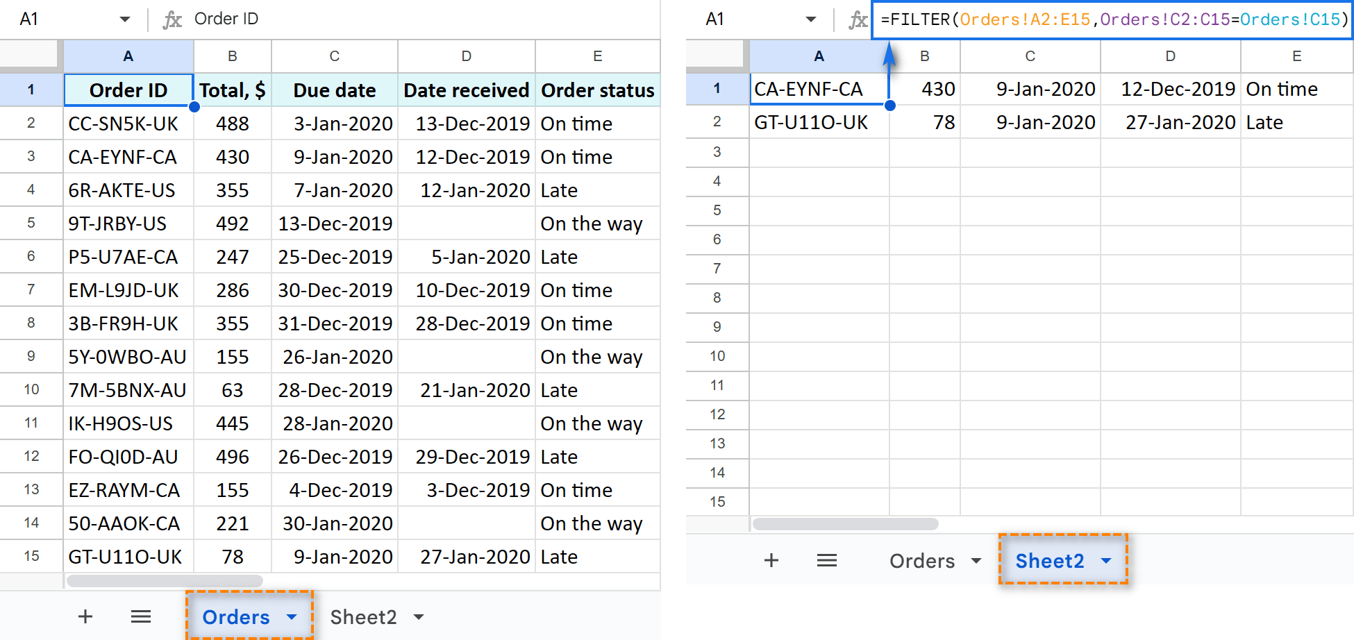
How do you filter from another Google sheet? I mean when your source table is on one sheet but you want to extract the result to another.
Easy — build the formula where you need to but bring the sheet name along every time you reference that another sheet :)
Here I create the formula on Sheet2 to have the filtered outcome there, but I refer to the Orders sheet since my original table is there:
=FILTER(Orders!A2:E15,Orders!C2:C15=Orders!C15)
Tip. If your sheet name has more than one word, wrap it in single quotation marks:
=FILTER('May orders'!A2:E15,'May orders'!C2:C15='May orders'!C15)
Filter from another Google file: Importrange
How do you filter from another Google file? Referencing just the sheet name is not enough, especially since it can be the same in your current file. So where do you put the name of the file?
Well, nowhere :) It's the link to that file you need, not its name.
IMPORTRANGE will help you with that:
- Your sheet name will become the second argument and you must wrap it in double quotes: "Orders!A2:E15"
- For the first argument, open the file with your original table, look at its URL and find its ID. It's a sequence of letters and numbers between /d/ and /edit:
https://docs.google.com/spreadsheets/d/1d5…8ww/edit#gid=0Put it to the formula in double quotes as well: "1d5…8ww"
Here's how your end formula for filtering from another Google file using IMPORTRANGE will look like:
=FILTER(IMPORTRANGE("1d5…8ww","Orders!A2:E15"),IMPPORTRANGE("1d5…8ww","Orders!E2:E15"&"=Late"))
Once you create the formula, the first thing you'll see is the #REF! error. No worries — it's IMPORTRANGE asking the permission to look at that file. Hover your cursor over the error and you'll see this explained on a special pop-up window:
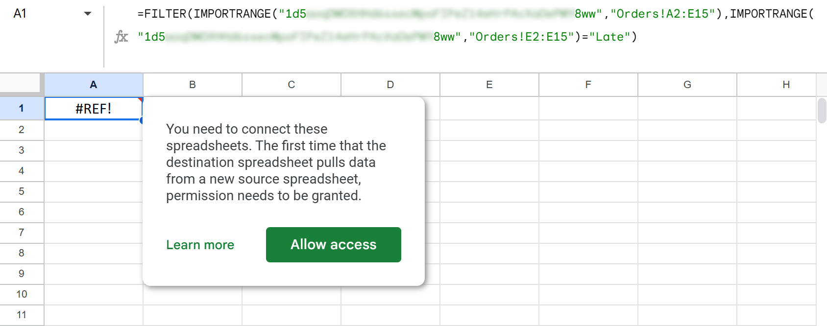
Hit the green Allow access button on the same window to connect the spreadsheets, and the formula will return only filtered rows:

Google Sheets FILTER function not working: solutions
Even the best of us may face roadblocks when working with the FILTER function in Google Sheets. Below I will cover the most common issues that may break your formula and provide solutions to get it back on track.
#REF! error
This one may hint at two things:
- Invalid cell references. Solutions? Check that you entered all ranges & all sheet names correctly. And just in case? Make sure the range still exists in your source table.
- IMPORTRANGE can't access the file. When filtering from another Google file using IMPORTRANGE, make sure you connect the function to that file as I described above. If this doesn't help, check both your file ID and if the file with that spreadsheet ID still exists.
#N/A error
You'll see this one if your FILTER formula couldn't find any matching results. A few reasons are possible requiring different solutions:
- Incorrect condition. Double-check your condition. It should be an exact match to whatever you're aiming for. Thus, looking for "On time" while the status is actually "Arrived" will result in this error.
- There are simply no matches. Once they appear, you'll see the filtered result. Or feel free to use some other condition instead right away 🙂
- Incorrect function name. That's right. While preparing the screenshots for this article, I had #N/A saying that FILTER has mismatched range sizes. I was on the verge of pulling my hair out trying to fix it (nothing worked because the ranges were OK) when I noticed I accidentally typed IMPORTRANGE with two Ps: IMPPORTRANGE! Correcting the name did the trick though 😎
#VALUE! error
If you see this error, chances are you use ranges of different sizes.
Remember, all conditions must have exactly the same length as a range. For example, if the range you want to filter ends with row 15 (A2:E15), the range in each condition should also end with row 15 (D2:D15<>"").
Also, check if your ranges with conditions consist of a single row or a single column, e.g. D2:D15<>"" rather than A2:E15<>"".
#NAME error
When filtering Google Sheets by color using custom formula, you may sometimes see this error. If you do, make sure you still have Function by Color.
Without it, the custom function won't work because it's not part of standard Google Sheets toolset.
Oh, and make sure your spreadsheet has a locale set up (File > Settings) since it controls function syntax.
Replace FILTER errors with your own text
If you don't care what error your Google Sheets FILTER returns and you'd rather see some custom text in your cells, the IFERROR function will help.
- value is your entire FILTER formula.
- [value if error] is whatever you want to see in cells when something goes wrong with the formula.
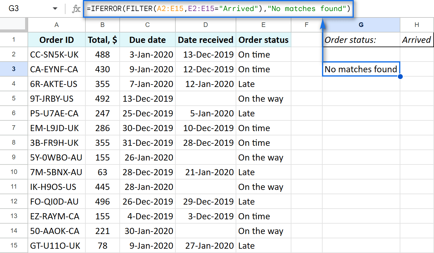
For instance, let's make it return "No matches found". Put the formula as the first argument, and the text in double quotes as the second one:
=IFERROR(FILTER(A2:E15,E2:E15="Arrived"),"No matches found")
If your error or case differs from those I described here, let me know in the comments!
Formula-free way to filter Google Sheets
FILTER function is great and all, but sometimes it can be too much. Keeping track of all arguments, delimiters, nested functions and whatnot can be extremely confusing and time-consuming.
Luckily, we have an ultimate solution that transcends both Google Sheets FILTER function and their standard tool. The add-on is called Filter and Extract Data.
It searches for and pulls matches to your conditions, but it's wa-a-ay easier than formulas ;)
I'll give you 5 reasons why this tool is better than the Google Sheets FILTER function:
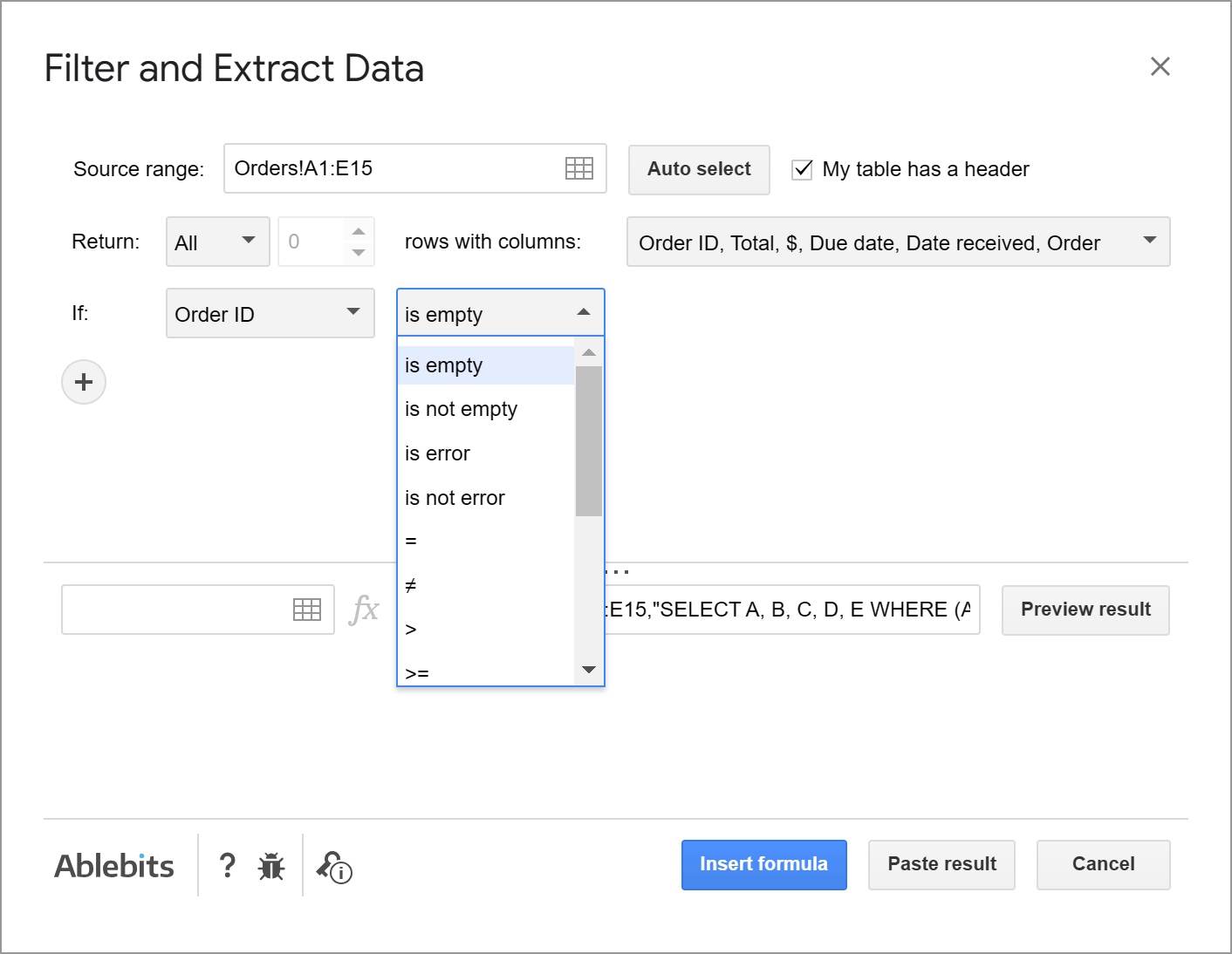
- You won't have to think about operators for different conditions — just pick the human word from the list:
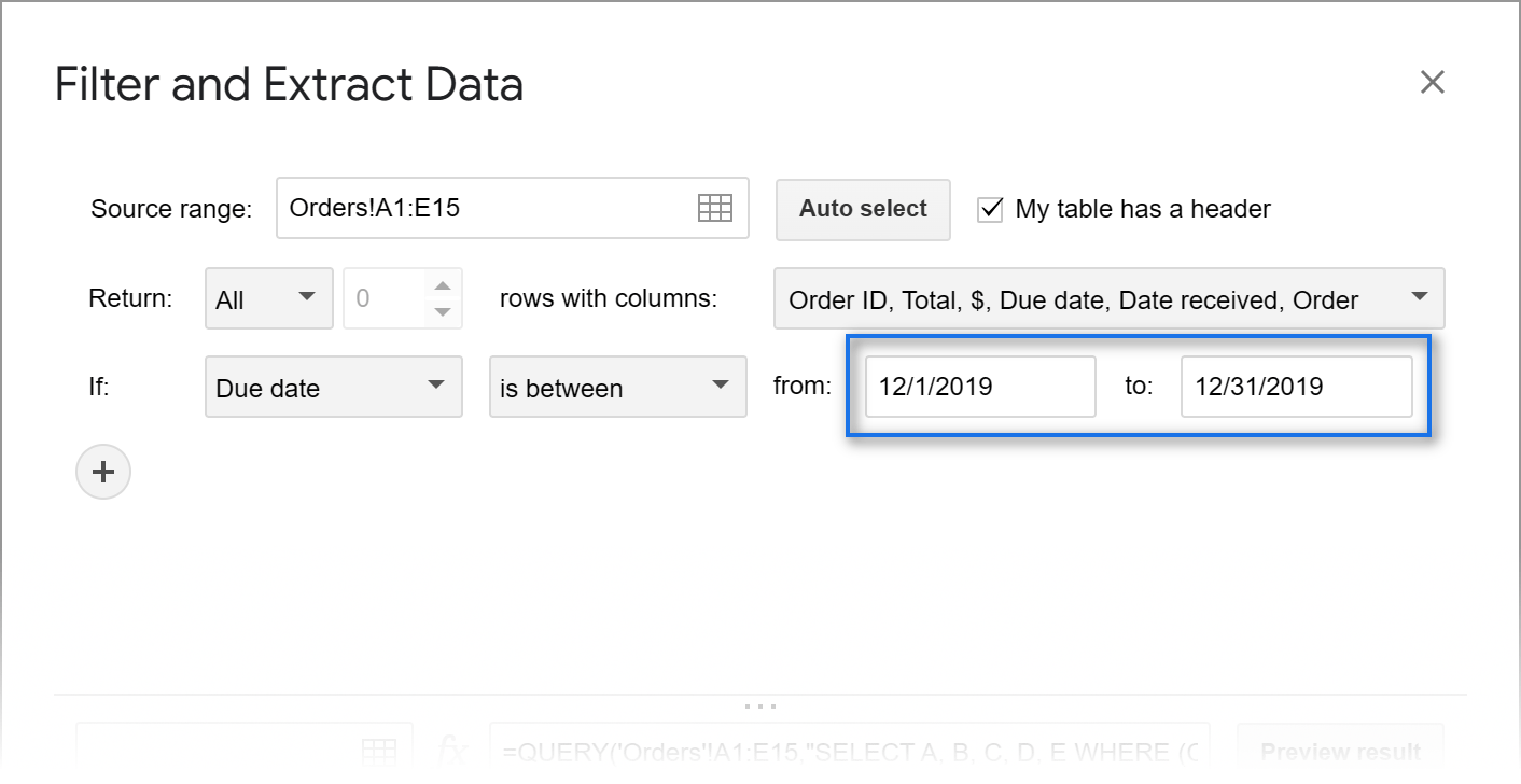
- Enter dates and time as you always do in spreadsheets — no more special MONTHS or HOUR functions:
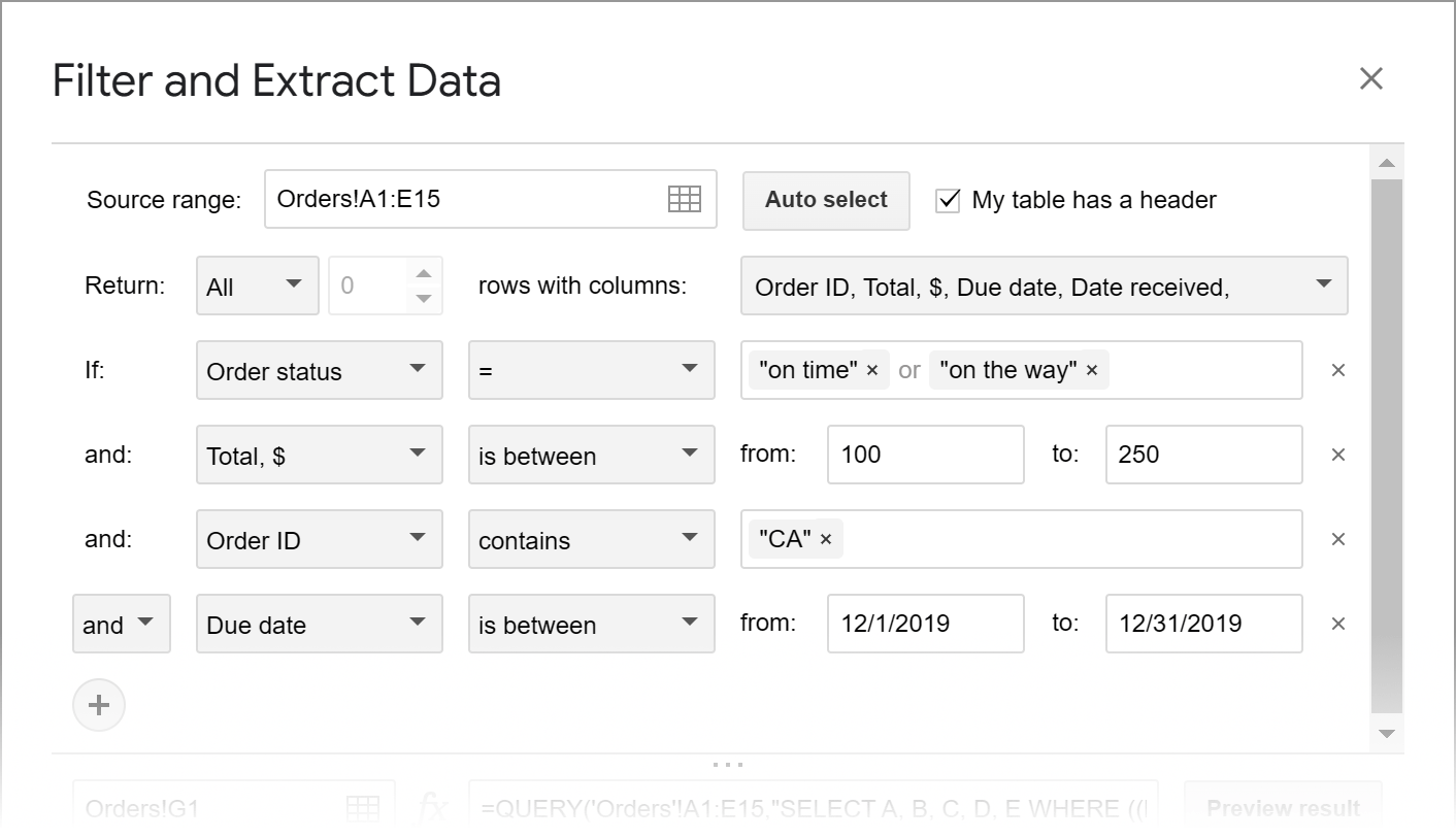
- Add and delete multiple conditions for multiple columns real quick:
- Preview the result and adjust conditions (if needed) before pasting everything to your sheet:
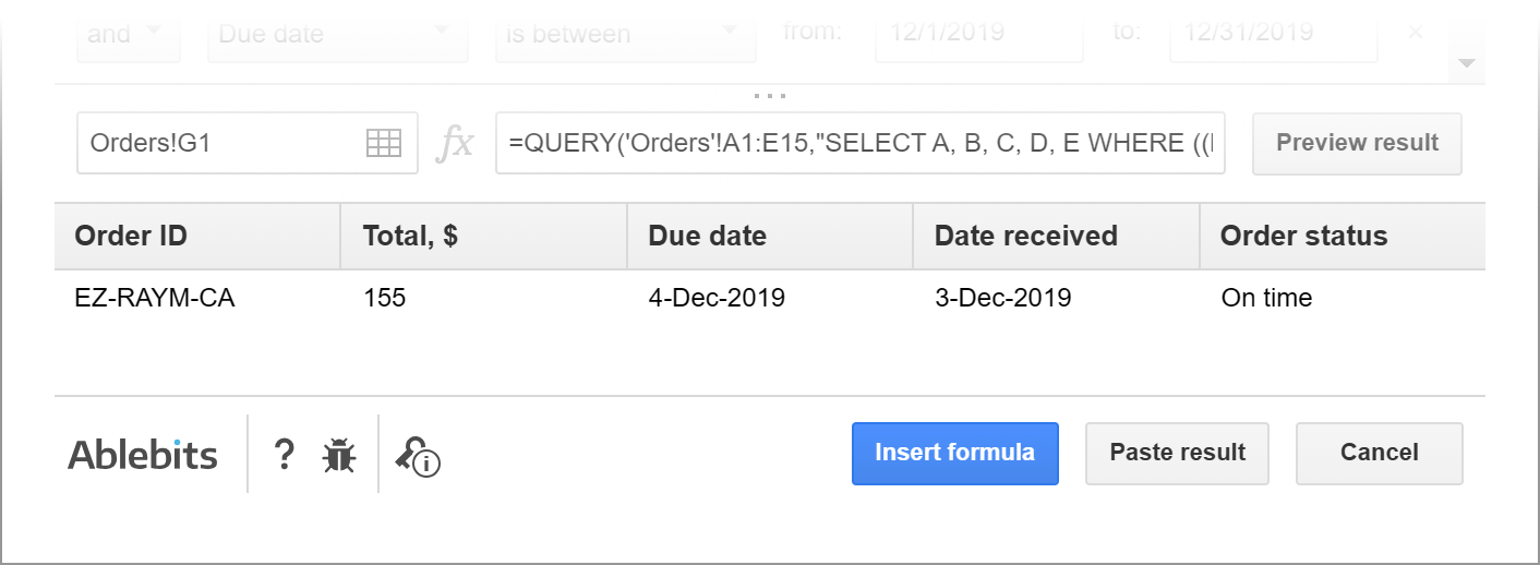
- Get the result as values or as a ready-made formula.
I truly encourage you to install Filter and Extract Data and give it a go.
To look through its options closer, visit its tutorial page or watch a special instructional video below.
Video: How to use Filter & Extract Data add-on for Google Sheets
Spreadsheet with formula examples
Google Sheets FILTER function (make yourself a copy)
 by
by 
45 comments
Jika saya ada kebutuhan untuk mengambil data hasil filter dari sheet berbeda (master database), rumus apa yang baiknya dipakai ya Bu sehingga pada sheet selanjutnya hanya ada tampilan hasil filter yang dipilih?
Terima kasih sebelumnya :)
Hello Priscilla,
You're on the correct page, I believe. The FILTER function from the above will help you out.
You can use the IMPORTRANGE function if your "Master Database" is in a different file/worksheet.
Hello,
I am trying to find all of the values that match my filter criteria in the top row. Whenever I to use the "match" formula in the first argument position in the "filter" formula I get an error stating that it must be a single range. (the member roster is on a separate sheet from where I am placing the formula)
=MATCH(C2,'Member Roster'!$A:$A,0) ANSWER IS 285
=TRANSPOSE(FILTER('Member Roster'!$1:$1,'Member Roster'!285:285=0,'Member Roster'!$1:$1"",ISTEXT('Member Roster'!$1:$1)))
Is there a work around for this?
Thanks!
I was able to answer my own question...
I had to make a prep cell to collect the column letter using:
This is in cell A3 → =concatenate(SUBSTITUTE(ADDRESS(1,column(index($N$1:$LF$1,1,match(A2,$N$1:$LF$1,0))),4),1,""))
then used a query to list the info the way I needed it
=query($L$1:$LG,"select L where "&A3&"=0")
Thank you for sharing your solution, Mike!
HI! I'm using the formula below and it's coming back with no results, however, there are 3 that match this criteria that aren't pulling in.
=FILTER(A4:H100,L4:L100="TRUE",B4:B100"")
Thoughts?
I'm using the below formula for another search and it's pulling correctly
=FILTER(D4:H100,C4:C100="New Style/Product",D4:D100"")
Hi Kayla,
Try removing double quotes from around TRUE. If it's a boolean value, it doesn't need double quotes as they're used for text only.
Hello! I am working on a sheet and I have two tabs. I am trying to filter data from THREE columns in one tab so that they show up in another tab but in a single column based on if there is data in the first tab. Is this possible? As of right now I can't get it to work properly.
This is the coding I'm currenly using. My problem area is "pending!M:O" - The formula is pulling the data I need, however, it's not inputting it into one column on the second tab, it's spreading them out which is making my 12 column sheet turn into a 15 column sheet.
=filter({Pending!F:F,Pending!G:G,Pending!H:H,Pending!M:O,Pending!L:L,Pending!I:I,Pending!J:J,Pending!P:P,Pending!Q:Q,Pending!D:D,Pending!E:E,Pending!K:K},Pending!B:B=true)
Basically, I need all information pulled from the Pending tab's columns M-O to popular in a single column on another tab instead of taking up three columns.
I hope I explained the issue clearly...
Thank you,
Breann
Hello Breanna,
For me to be able to help you, please consider sharing an editable copy of your file (including your formula) with us: support@apps4gs.com. If you have confidential information there, you can replace it with some irrelevant data, just keep the format.
Note. We keep that Google account for file sharing only and don't monitor its Inbox. Please do not email there. Once you share the file, just confirm by replying to this comment.
Input =FLATTEN(FILTER(your entire formula above))
I hope it works.
Hello,
I am currently trying to filter data from sheet1!A2:K506 with the condition that sheet1!E2:E506 is equal to B1 and F2:F506 is "Yes".
I have tried using:
=FILTER(sheet1!A2:K506, (sheet1!E2:E506=B1)+(F2:F506="Yes"))
But it came back with an error.
Appreciate if you can let me know the solution if you have any.
Thank you!
Apologies, it should be sheet1!F2:F506.
Hi!
If you use multiple conditions that are combined with "and" logic, use multiplication in the formula, not summation.
=FILTER(A2:K506,(E2:E506=$B$1)*(F2:F506="yes"))
I hope my advice will help you solve your task.
Hi there! I have a situation. I have a table with fields that may contain a date, a month and a year respectively. These fields may also be blank. I want to use them as a filter for an array that copies an existing table from another sheet. The original table has a date column. I want to filter the table copy by date, month or/and year properly so that when I change the values of those filter fields the clone table would also be updated. And I also don't want to apply the filters when they are empty (e.g. in this case I would get the same table as the original one).
Example:
original table
Date Value
01/02/2022 v1
03/04/2021 v2
copy table
filters
Date filter Month filter Year filter
(empty) 2 2022
filtered result
Date Value
01/02/2022 v1
Can anyone please help? Thanks in advance.
- Iliyan
P.S.: I would very much like to do this with the FILTER() function or some formula. So far I am not able to make it this way.
Hi Iliyan Tenev Iliev,
Please consider sharing an editable copy of your spreadsheet with us (support@apps4gs.com) with 2 sheets: (1) a copy of your source data (2) the result you expect to get. I kindly ask you to shorten the tables to 10-20 rows.
Note. We keep that Google account for file sharing only and don't monitor its Inbox. Please do not email there. Once you share the file, just confirm by replying to this comment.
I'll look into and try to help with a formula.
Hello Good day to all,
i have invoice sheets that i constantly monitoring and i am having trouble with the two column, one is invoice # (B16:B) and revised invoice # (C16:C), and made a search sheet were i can search BY PO, BY DATE etc., what i want is when i type or search for the invoice number it will search within those two column (invoice # (B16:B) and revised invoice # (C16:C)) and will return the desired outlput
Im using the following formula :
=filter(Invoices!$A$16:$U,search($A$2,Invoices!$B$16:$B),search($B$2,Invoices!$D$16:$D),search($C$2,Invoices!$F$16:$F),search($D$2,Invoices!$G$16:$G),search($E$2,Invoices!$S$16:$S))
am I missing something? please help, thank you
Hello Exequiel Jr.,
As far as I can see, your current formula misses column C16:C at all. If you need to check whether your number appears at least in one of the columns (OR logic), this part of the blog post (Example 2) should help.
Hi there,
Thanks for this super helpful resource, it has helped me to get a hold of just how much we can achieve with filtering. I have a question about whether it is possible to filter for the same condition from two different sheets in the same Google Sheet. I tried applying the OR logic as above but it is returning a VALUE error message, I've copied the formula I tried below.
=FILTER('IA'!C2:F5,'IA'!C2:C5="Family activity packs")+('SF'!C2:F5,'SF'!C2:C5="Family activity packs")
Any help would be gratefully received.
Hi Ian,
Thank you for your lovely feedback!
Try this formula instead:
={FILTER(IA!C2:F5,IA!C2:C5="Family activity packs");FILTER(SF!C2:F5,SF!C2:C5="Family activity packs")}
.thanks, and sorry to bother you again Is the connection between drop list and table possible in this situation .if i have created a drop down e = azam, nazam, shazam which is the content of b column, and i want A C E column based on drop down list. how its possible with power query ...mam help me please
Sorry """ from above question i need A C D column based on drop down list
Hi again,
Sure, it's possible. Try to use a condition like this: 'QUERY(..., "select A,C,E where B=E1")
Assuming, your drop-down is in E1.
You'll find more examples and ready-made formulas on the blog post devoted to QUERY.
hi mam, Sorry to bother again,
i did the same thing but its showing error, i applied 'QUERY(Range "select A,C,D where B=E1")
where Column B unable to take reference Cell E1,,,
im try trying but its showing error...
Hi Saaha,
There should be a comma right after your range, before "select...". If it doesn't help, for me to be able to help you better, please share an editable copy of your spreadsheet with us (support@apps4gs.com). Make sure to highlight the QUERY formula you created so I could see where to look.
Note. We keep that Google account for file sharing only and don't monitor its Inbox. Please do not email there. Once you share the file, just confirm by replying to this comment.
Hi Mam,
i've sent you sheet copy to you through mail. sorry actually i ve sent you same file twice, and file name is" Saaha file to resolve file to resolve filter problem" Please go through
Thank you for sharing the spreadsheet, Saaha.
I've fixed your formula directly in there, please have a look.
Thank you so much mam,
i was waiting for your reply , and you are so humble, you guys are always help us,
and thank you again Mam..????
You're most welcome, Saaha! :)
if there are 5 column i.e A B C D E but i want to filter only A C E so how could we use filter formula for this condition please give me formula
if there are 5 column i.e A B C D E but i want to filter only A C E so how could we use filter formula for this condition please give me formula, I dont want entire column i just need information of A C E where B=L4 please help me
Help me i want to filter only A C E so how could we use filter formula for this condition please give me formula, I dont want entire column i just need information of A C E where B=L4 please help me
Hello Saaha,
If you'd like to return only part of the columns based on the contents of some of them, you'd better use the QUERY function instead.
thanks alote , and sorry to bother you again if i have created a drop down list E4 = azam, nazam, shazam which is the content of B column, and i want A C E column based on drop down list , Its possible with the power query or filer formula and How ?? Is the connection between drop list and table possible in this situation please give me a formula?
Please help me
Please help me im waiting for your reply??!!!!!!!!!!!!!!!!!!
Saaha,
I replied to your comment above, please take a look.
Actually, you can do this with the Filter function directly! You don't need to use Query
e.g. =FILTER({C:C,B:B},D:D>=2)
THANKS!!!!
Thank you so much for posting the note on how to use OR logic with a filter function. For as practical a use case as that is, I don't see this anywhere else on the internet and I can't imagine who would have figured this out intuitively. This saved me hours.
Hi there,
I am trying to use the Filter function to snag data from another tab. This is the formula that I have, = FILTER(Artists!A:D,Artists!E:E= "yes").
I would like to be able to insert new columns into the Artist sheet between column D and E without the FILTER formula changing. I tried adding Absolute References to the formula like so, = FILTER(Artists!A:D,Artists!$E:$E= "yes"), but when I Insert a column in the Artist sheet between column D and E, the FILTER function changes to Artists!F:F (or Artists!$F:$F).
Is there anyway to use absolute references within the FILTER function so it doesn't update when new columns are added?
Paul
Hi Paul,
Formulas in Google Sheets are dynamic. If you refer to a particular range/column and then insert new cells/columns causing your original range change letters, ranges/columns in formulas will change accordingly. This way your formulas will always refer to the same range and don't break.
The only way to make the formula always use the contents of a particular column is to reference it with the INDIRECT function.
Thanks! I ended up finding the INDIRECT function a few hours after posting. Thanks for confirming that I did it right. :)
My pleasure, Paul!
Hi Natalia, I have been trying to combine two of the concepts you outlined with a little trouble. I am trying to filter where text 'contains' multiple conditions in one column. So here is what I have:
=FILTER($WO3:$W,(SEARCH("Sub",$R3:$R))+(SEARCH("Viv",$R3:$R)))
I am trying to display columns O through W filtering for column R containing either 'Sub' or 'Viv', but all I get is #N/A stating there are no matches. I am attempting to combine the two examples you provided:
=FILTER(A1:E20,SEARCH("ca",A1:A20,8))
=FILTER(A1:E20,(E1:E20="Late")+(E1:E20="On the way"))
Let me know if this is possible, thank you!
Hi Jason,
Your formula doesn't work because SEARCH returns errors for all rows that don't have 'viv' or 'sub'. Wrap those SEARCH formulas into IFERROR and it'll work:
=FILTER($WO3:$W,IFERROR(SEARCH("Sub",$R3:$R))+IFERROR(SEARCH("Viv",$R3:$R)))