Every once in a while each Google Sheets user faces the inevitable: combining several sheets into one. Copy-pasting is tedious and time-consuming, so there has to be another way. And you're right — there are several ways, in fact. So get your tables ready and follow the steps from this article.
All the ways I describe can be used to process large tables. But to keep this guide as clear as possible, I'll keep my tables short and am going to cut down to a couple of sheets.
Reference cells in Google Sheets to pull data from another tab
The easiest way comes first. You can pull entire tables to one file by referencing cells with data from other sheets.
Note. This will do if you need to merge two or more sheets within one Google spreadsheet. To merge multiple Google spreadsheets (files) into one, jump right to the next method.
So, my data is scattered all over different sheets: June, July, August. I'd like to pull data from July and August into June to have one table as a result:
- Find the first blank cell right after your table (the June sheet for me) and place the cursor there.
- Enter your first cell reference. The first table I want to retrieve starts from A2 in the July sheet. So I put:
=July!A2Note. If there are spaces in your sheet name, you must wrap it in single quotes like this:
='July 2022'!A2This immediately replicates whatever lies in that cell:

Note. Use relative cell reference so it changes itself when copied to other cells. Otherwise, it will return incorrect data.
- Make sure the cell with the reference is selected and click on that little blue square at its bottom right corner. The mouse cursor will turn into a big black plus sign. Keep the mouse pressed and drag the cursor to as many columns to the right as you need to fill them with new records:

- Select this entire new row, click that little blue square once again, hold and drag your mouse down — this time to fill entire rows with cell references and bring new data from another sheet:
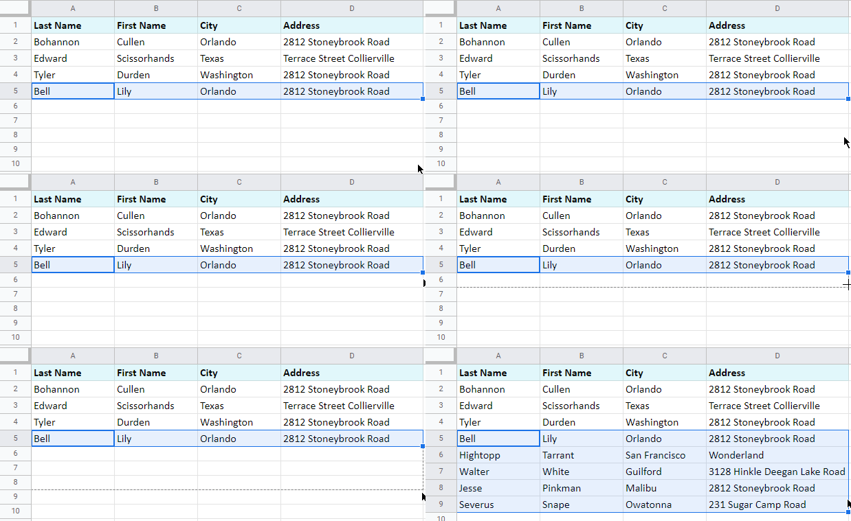
Though this is probably the first way you may think of to pull data from another tab, it's not the most elegant and quick. Luckily, Google prepared other instruments specially for this purpose.
Copy the tabs into one spreadsheet
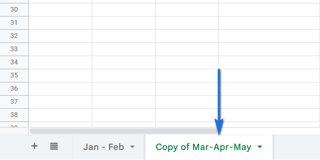
One of the standard ways is to copy the tabs of interest into the destination spreadsheet:
- Open the file that contains the sheet(s) you want to transfer.
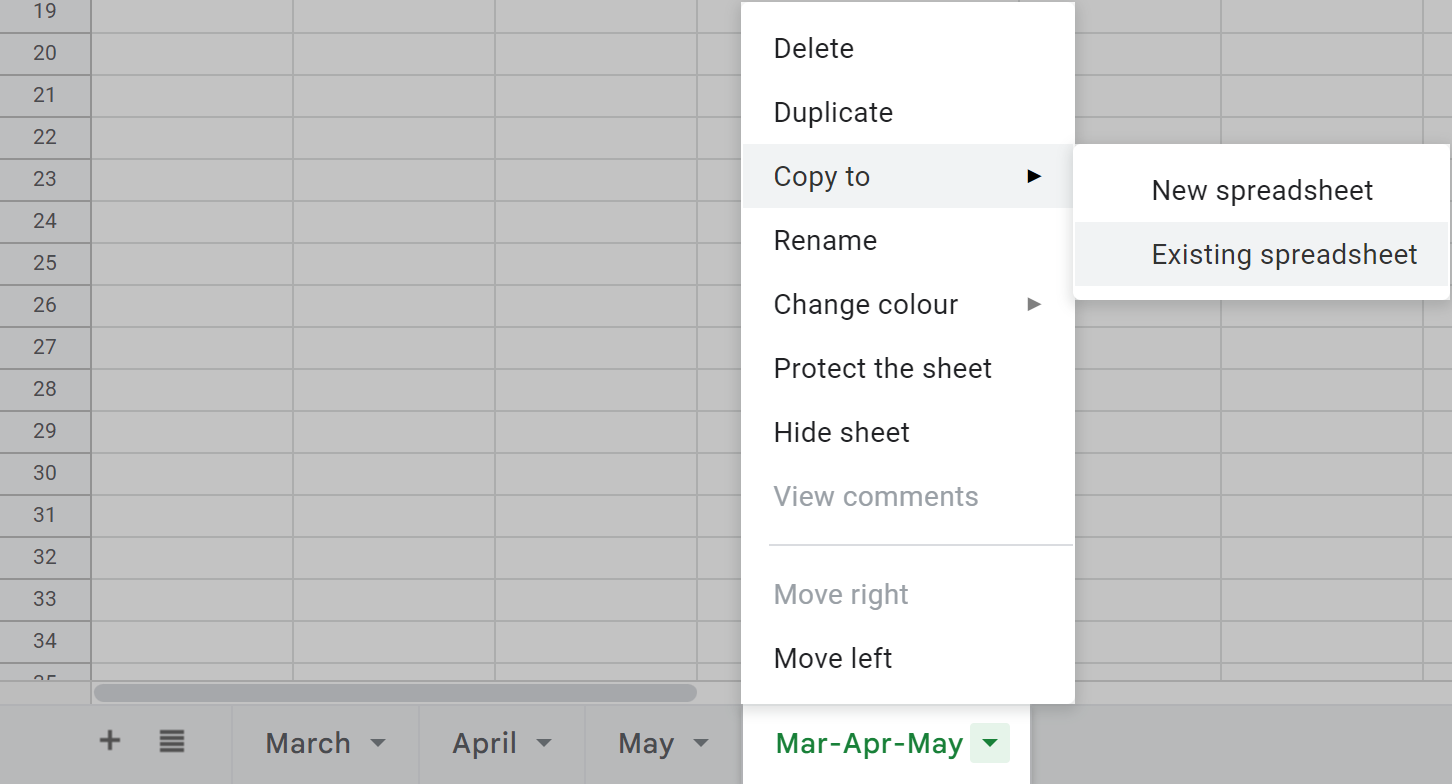
- Right-click the first tab you need to export and choose Copy to > Existing spreadsheet:
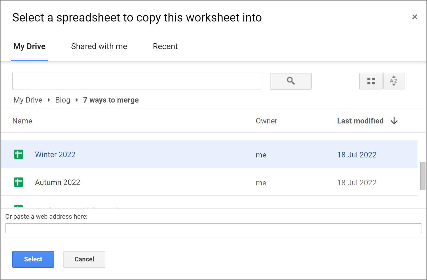
- The next thing you'll see is the pop-up window inviting you to select the spreadsheet. Browse for it, click on it to highlight it, and press Select when you're ready:
- Once the sheet is copied, you'll get a corresponding confirmation message:

- You can either hit OK and continue with the current sheet or follow the link called Open spreadsheet. It will instantly get you to another spreadsheet with the first sheet already there:
Export/import sheets
Another way to import data from multiple Google Sheets is to export each sheet first, and then import them all to a necessary file:
- Open the spreadsheet that contains the sheet you'd like to pull the data from.
- Make the sheet of interest active by selecting it.
- Go to File > Download > Comma-separated values (.csv):
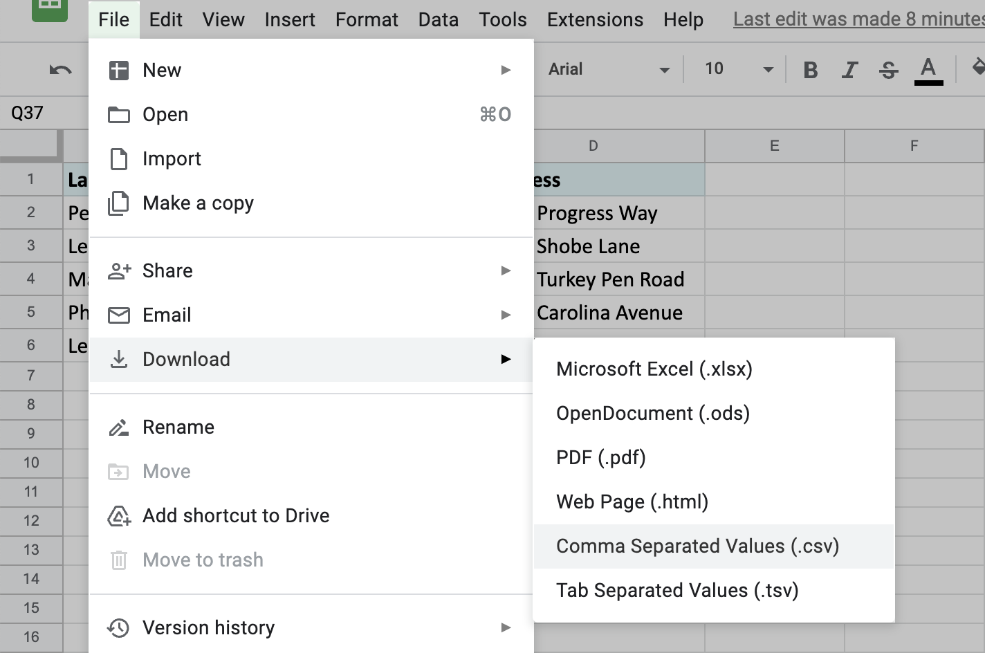
The file will be downloaded to your computer.
- Then open another spreadsheet — the one you'd like to add the sheet to.
- This time, pick File > Import from the menu and go to the Upload tab in the Import file window:
- Hit Select a file from your device and find the sheet you've downloaded just now.
- Once the file is uploaded, you'll see a window with additional options for importing the sheet. To add the contents of that another sheet after your existing table, pick Append to current sheet:
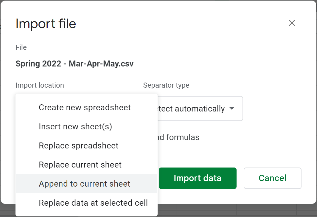
Tip. Among other settings, feel free to specify the separator and convert text to numbers, dates, and formulas.
- As a result, you'll get two sheets merged — one table under another:
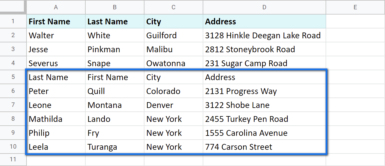
But since it is a .csv file you need to import, the second table remains formatted in a standard way. You will have to spend some time formatting it as you need.

Google Sheets functions to combine data from multiple spreadsheets
Of course, it wouldn't be Google if it didn't have functions to merge data in Google Sheets.
IMPORTRANGE to import data from multiple Google sheets
As the name of the function suggests, IMPORTRANGE imports data from multiple Google spreadsheets into one sheet.
Tip. The function helps Google Sheets pull data from another document as well as from other tabs from the same file.
Here's what the function requires:
- spreadsheet_url is nothing else than the link to the spreadsheet from where you need to pull the data. It must always be put between double-quotes.
- range_string stands for those cells specifically that you need to bring to your current sheet.
And here's the pattern I follow to import data from multiple Google Sheets using IMPORTRANGE:
- Open the spreadsheet from which you want to pull the data.
Note. Make sure you have at least viewing access to that file.
- Click the browser URL bar and copy the link to this file right till the hash sign (#):
- Return to the spreadsheet where you want to add the info to, enter the IMPORTRANGE to where the borrowed table should appear, and insert the link as the first argument. Then separate it from the next part with a comma:
- For the second part of the formula, type in the name of the sheet and the exact range that you want to pull. Confirm by pressing Enter.
Note. Wrap the second argument in double quotes as well:
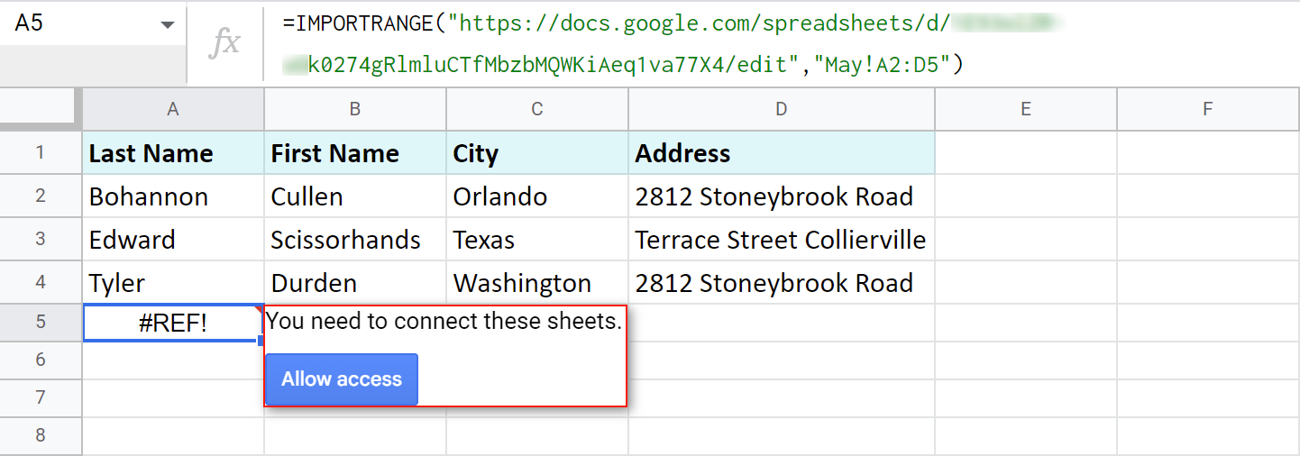
=IMPORTRANGE("https://docs.google.com/spreadsheets/d/XYZk0274gRlmluCTfMbzbMQWKiAeq1va77X4/edit","May!A2:D5") - Though the formula looks ready now, it will return the #REF error from the start. That's because the first time you try to pull data from some spreadsheet, IMPORTRANGE will ask for access to it. Once the permission is granted, you will easily import records from other sheets of that file.
Click the cell with the error and press that blue Allow access prompt:
- Once the formula connects to that other sheet, it will import data from there:
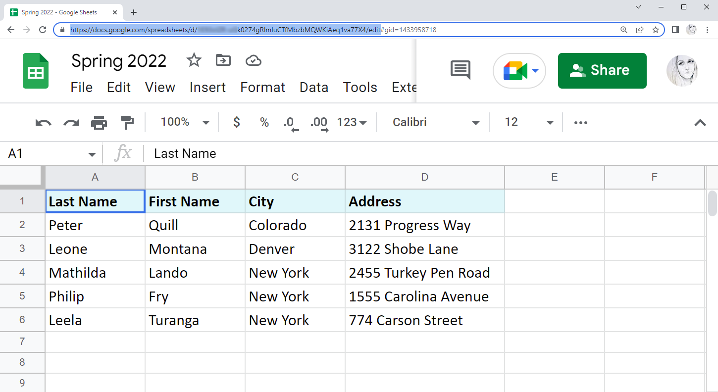
Note. You'll need this URL even if you're going to combine sheets from the same file.
Tip. Though Google says the function requires the whole URL, you can easily get by with a key — a part of the URL between /d/ and /edit:
...google.com/spreadsheets/d/XYZk0274gRlmluCTfMbzbMQWKiAeq1va77X4/edit

Note. Remember, the link should be surrounded by double quotes.
Note. By allowing access, you let the Sheets know you don't mind any existing or potential collaborators on this spreadsheet accessing data from another file.
Note. IMPORTRANGE doesn't pull the formatting of the cells, only values. You will need to apply formatting manually afterwards.
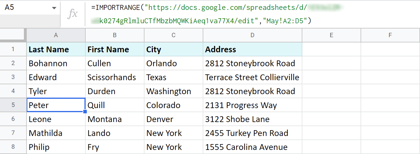
Tip. If the tables are rather big, just allow some time for the formula to pull all records.
Note. The records returned by the function will be updated automatically if you change them in the original file.
Google Sheets QUERY to import ranges from multiple sheets
And thus, without haste, we've come to the QUERY function once again. :) It is so versatile that can be used in Google spreadsheets to combine data from multiple sheets (within the same file) as well.
So, I want to merge three different Google sheets (from one file): Winter 2022, Spring 2022, and Summer 2022. They contain the names of all employees who became best in their jobs in different months.
I go to the first sheet — Winter 2022 — and add my QUERY right under the existing table:
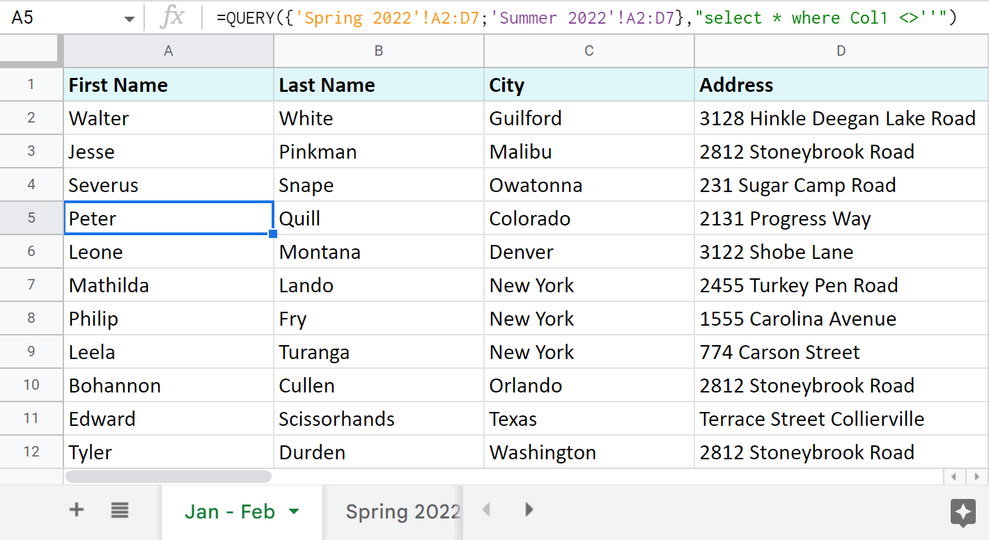
=QUERY({'Spring 2022'!A2:D7;'Summer 2022'!A2:D7},"select * where Col1 <>''")
Let's see what it all means:
- {'Spring 2022'!A2:D7;'Summer 2022'!A2:D7} — are all the sheets and ranges I need to import.
Note. The sheets should be written in between the curly brackets. If their names contain spaces, use single quotes to list the names.
Tip. Separate the ranges with a semicolon to pull data from different tabs one under another. Use commas instead to have them imported side by side.
Tip. Feel free to use such infinite ranges as A2:D.
- select * where Col1 <>'' — I tell the formula to import all records (select *) only if cells in the first column of the tables (where Col1) are not blank (<>''). I use a pair of single quotes to indicate the non-blanks.
Note. I use <>'' because my column contains text. If your column contains other data type (e.g. date or time, etc.), you need to use is not null instead: "select * where Col1 is not null"
As a result, two tables from other sheets have been consolidated into one sheet one under another:
Tip. If you'd like to use Google Sheets QUERY to import ranges from multiple separate spreadsheets (files), you will have to implement IMPORTRANGE. Here's a formula to pull your data from other documents:
=QUERY({IMPORTRANGE("XYZk0274gRlmluCTfMbzbMQWKiAeq1va77X4","Mar-Apr-May!A2:D6");IMPORTRANGE("XYZahJZHSlhMGLSW_xA6ZBqNmt1I0ADo4N4M","Jun-Jul-Aug!A2:D4")},"select * where Col1<>''")
Tip. I use the keys from URLs rather than entire links in this long-enough formula. If you're not sure what that is, please read here.
Tip. You can also use QUERY to merge two Google sheets, update cells, add related columns & non-matching rows. Check this out in this blog post.
3 quickest ways to merge multiple Google sheets
If standard ways of Google spreadsheets to combine data from multiple sheets seem dull, and the functions scare you off, there's an easier approach.
Combine Sheets add-on
This first special add-on — Combine Sheets — was designed with a single purpose: import data from multiple Google sheets.
It's clever enough to recognize the same columns in different sheets and bring data together accordingly if you need.

All you are to do is:
- Select sheets or entire spreadsheets to merge and specify the ranges if necessary. A quick search across your Drive makes this even faster.
- Choose how to pull the data:
- as a formula. Mark the checkbox called Use a formula to combine sheets if you want to have a master sheet that will dynamically change based on your original contents.
Although you won't be able to edit the resulting table, its formula will be always linked to the source sheets: edit a cell or add/remove entire rows there, and the master sheet will be altered accordingly.
- as values. If editing the resulting table manually is more important, ignore the above option and all data will be combined as values.
Extra options are here for fine-tuning:
- join records from the same columns into one column
- keep the formatting
- add a blank line between different ranges to notice them right away
- as a formula. Mark the checkbox called Use a formula to combine sheets if you want to have a master sheet that will dynamically change based on your original contents.
- Decide where to place the merged table: new spreadsheet, new sheet, or in a location of your choice.
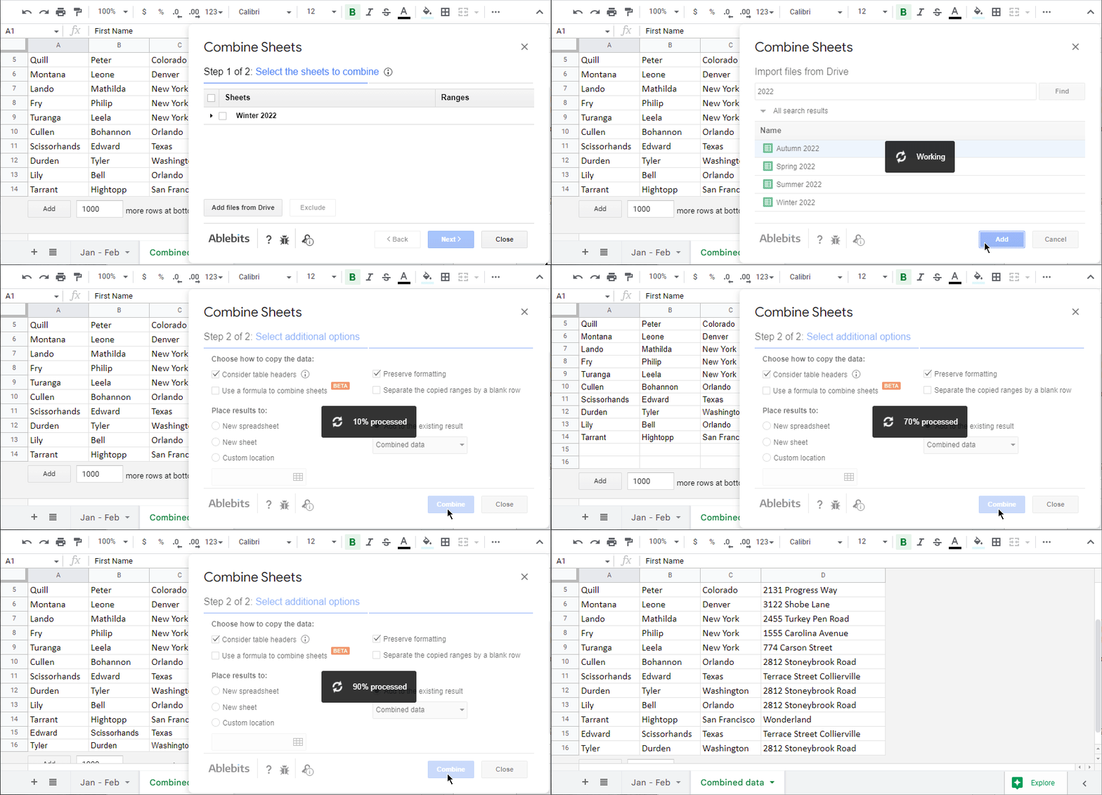
Here's a quick demonstration of how I combined my three small tables with the add-on:
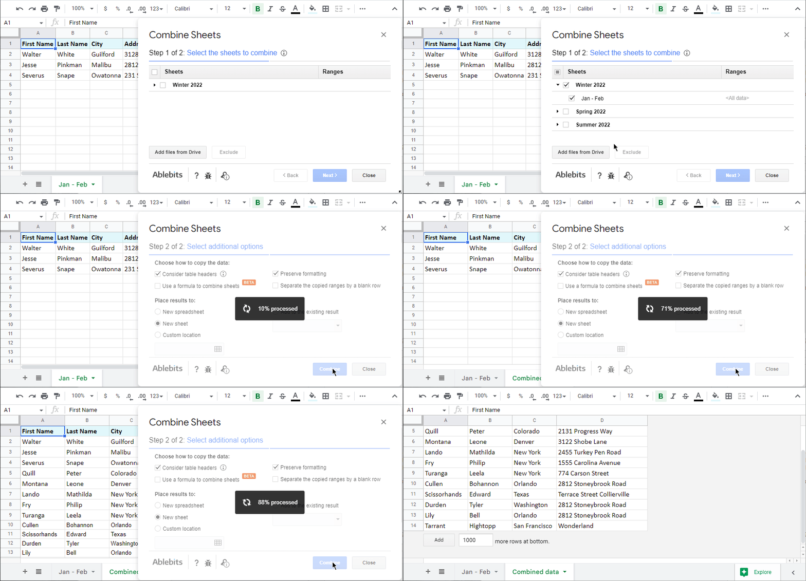
Of course, your tables can be much bigger and you can merge lots of different sheets as long as the resulting file doesn't exceed the 10M cell-limit.
One of the options this add-on offers is to add more sheets to your previously combined data. In this case on step 1, you need to pick not only the data to combine but also the existing result. Here's how it looks:
Video: How to combine multiple Google sheets into one
Check out the help page for Combine Sheets or watch this 3,5-minute tutorial:
Consolidate Sheets add-on
Consolidate Sheets is another handy tool among our add-ons. Its main difference from the aforementioned tool is the ability to add up data in columns in Google Sheets (or rows, or single cells, for that matter).
Consolidate Sheets also recognizes common headers in all the Google sheets to join, even if they are in the leftmost column and/or the first row. There's always an option to merge Google sheets and calculate cells based on their place in the tables.
Let me break it down into steps for you as well:
- Select sheets to consolidate. Import more files from Drive if necessary straight from the add-on.
- Pick the function to consolidate in Google Sheets.
- Choose the way to add up cells in Google Sheets: by labels (header labels, left column labels, or both) or position.
- Decide where to place the consolidated data: new spreadsheet, new sheet, or any specific location within the opened file.
Here's how this process looks:
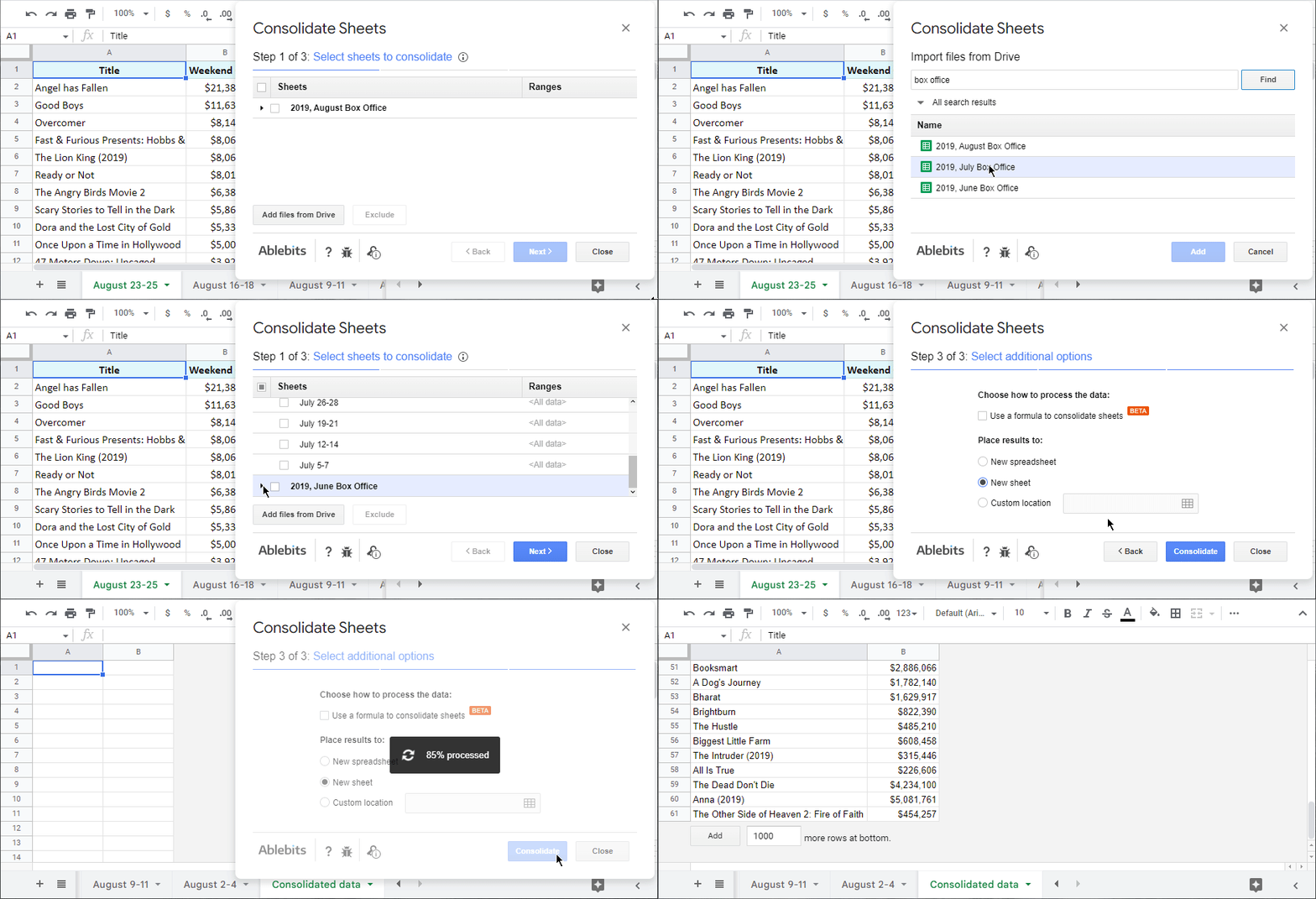
There's also an option to consolidate all your sheets using a formula. This way your result will change in sync with the values in the source sheets:
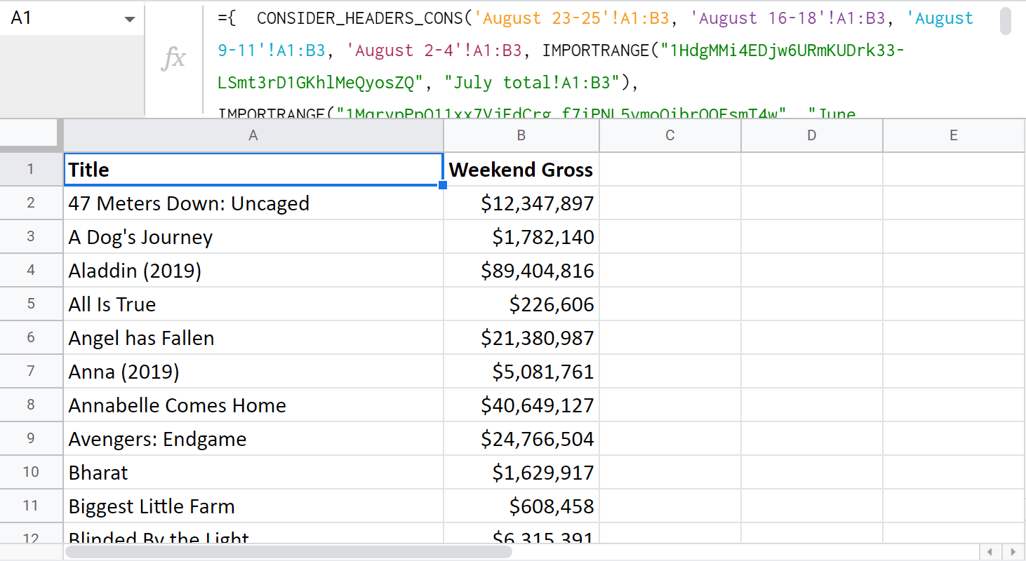
Note. There are some peculiarities you need to know about how the formula works. For example, if you consolidate from multiple different files, there will be an extra step to connect the sheets for the IMPORTRANGE in use. Please visit the instructional page for Consolidate Sheets for these and other details.
Video: How to consolidate multiple Google sheets into one
Here's a 4-minute demo-video about the add-on work:
I truly encourage you try this add-on. You'll see for yourself how much extra time you'll have after incorporating this tool to your daily work.
Merge Sheets add-on
There's one more add-on worth mentioning — Merge Sheets. It matches records from the same column in several sheets/documents and then pulls related data from the lookup sheets/documents into the main one. Hence, you always have an up-to-date spreadsheet at hand.
There are 5 straightforward steps:
- Select your main sheet.
- Select your lookup sheet (even if it's in another spreadsheet).
- Choose columns where matching records may occur.
- Tick of the columns with records to update.
- Tweak any additional options that will help you merge two sheets and achieve the best result possible.
You can even save the settings into reusable scenarios and run them later in a click.
Video: How to merge Google sheets
I know a picture is worth a thousand words, so here's a 3-minute video tutorial on Merge Sheets for you:
Ready to try it for yourself?
or visit this help page for details about each step and setting.
On this note, I'm going to finish this article. Hope these ways of pulling data from multiple different sheets into one will be of use. As always, looking forward to your comments!
 by
by 
220 comments
Hello!
I am trying to merge data from 6 different spreadsheets into one using the QUERY and IMPORTRANGE formula from above. I can get the formula to pull the data in for 1 spreadsheet at a time, but I receive an error when I try multiple spreadsheets. The data I'm trying to pull is in Columns A to H from each spreadsheet for a complete view of the data in one location. I even copied and pasted the formula you have above and added in my links and the range for each spreadsheet. Can you help?
Thanks!
Hello Amanda,
What error are you getting exactly? What does it say when you hover your mouse over it?
I had yesterday off and now trying to remember the exact thing I did. At first, I received the error "In ARRAY_LITERAL, an Array Literal was missing values for one or more rows". I changed something, and now I'm receiving the "Formula parse error". Here are the formulas for each:
ARRAY_LITERAL
=QUERY({importrange("MaGf45LzhXNrWcbLWG-e63R6PyTSor2Lbo", "Line Items!A2:H84"); importrange("1xDq2h28ZgI3aahyrIp7rihKq78K9wM79MFKwRKf3ACg", "MW FY25!A11:H30")},"select*where Col1 is ''")
PARSE
=QUERY({IMPORTRANGE("1bvgoJHOl-MaGf45LzhXNrWcbLWG-e63R6PyTSor2Lbo","Line Items!A2:H82"),IMPORTRANGE("1xDq2h28ZgI3aahyrIp7rihKq78K9wM79MFKwRKf3ACg","MW FY25!A11:H30"}),"select * where Col1''")
Hello Amanda,
The 'In ARRAY_LITERAL' error occurs whenever there is a sheet with only a header row among your original tables. Will you be able to check that?
Also, the criteria in your second formula is incorrect. Try "select * where Col1 = ''"
If neither solution helps, for me to be able to help you better, please consider sharing your spreadsheet with a formula and spreadsheets you're trying to merge with me directly: support@apps4gs.com
Note. We keep that Google account for file sharing only and don't monitor its Inbox. Do not email there. Once you share the file, just confirm by replying to this comment.
I'll look into it and try to help.
Hi,
Hope you are doing well.
You have mentioned: "There's also an option to consolidate all your sheets using a formula. This way your result will change in sync with the values in the source sheets".
Is it possible to provide me the formula as it will be very helpful for my project. Also, please guide me on how this formula can be executed as a function in Apps script.
Thank you in advance.
Hi Chetana,
It is the Consolidate Sheets add-on that creates this formula. Just install the tool from Google Workspace Marketplace and select the option 'Use a formula to consolidate sheets' on step 3.
Can I simply just say what a relief to discover an individual who really knows what they're talking about over the internet. You certainly know how to bring a problem to light and make it important. A lot more people really need to check this out and understand this side of your story. It's surprising you aren't more popular since you certainly possess the gift.
Hi! I'm looking to create a roll-up tab from 24 unique tabs all within one Google Sheets workbook. Each individual tab contains data populated by the Google Analytics report builder. I am unable to add any unique identifying data in each tab as every time the reports are updated, all added formulas are wiped.
Is there a way using any of the the abovementioned methods to create a dynamic roll-up using formulas AND somehow adding a column that identifies which tab the data comes from?
For example, for each row of data, how can I include the tab name in a new column?
Hi Jac,
If I understand you correctly, Combine Sheets add-on will help you. It can use a formula to combine sheets so the result is updated each time something changes in the original tables.
We're also currently working on adding the feature that will enable Combine Sheets add sheet name in a new column to the right. There's no other native way for that, I'm afraid, only using Apps Script.
Hi,
I have a schedule for appointments that is broken out into two tabs. On the first tab, the names of people on the schedule are chosen from a drop down in column A. Once a person is selected, their address is automatically populated into columns B-D. The services they receive are manually chosen from drop downs in columns E, F, and G. The second tab pulls columns A-D into it via an importrange formula. A different set of services are chosen in columns E-G on this tab. I basically want to be able to delete and rearrange rows in Tab 1 and have the entire row in Tab 2 do the same thing. Right now, only the cells referenced in the importrange change, which makes sense, but it's not what I would like to have happen. Is there a way to accomplish this? Thank you!
Hi Christy,
I'm sorry but your task is not entirely clear. For me to be able to help you, please share a small sample spreadsheet with us (support@apps4gs.com) with (1) a copy of your source data (2) the result you expect to get. I kindly ask you to shorten the tables to 10-20 rows.
Note. We keep that Google account for file sharing only and don't monitor its Inbox. Do not email there. Once you share the file, just confirm by replying to this comment.
I'll look into your task and try to help.
Thank you, Natalia. I have shared my sample file.
Thank you for sharing the file, Christy.
I'm afraid that those portions of data that are not connected by a formula to the first tab or to the first columns should be managed manually. There's just nothing that connects them, you see. You can at least extend your IMPORTRANGE to column D as B-D are automatically populated on the first tab as you mentioned in your first comment.
I should also note that IMPORTRANGE returns blanks from the range as well. If I remove Johnny Appleseed, there are 2 blank cells in-between other records that IMPORTRANGE returns. You may want to try and wrap IMPORTRANGE in QUERY to pull only those rows where A is not blank. Our Filter and Extract Data add-on will help you built the correct formula as well.
Hi
is there any way in google sheets to reference data from multiple sheets without specifically referencing each one?
In excel you can refer to ranges of sheets, e.g. =sum(Jan:Dec!A1) would add cell A1 from all the sheets between 'Jan' and 'Dec' in a workbook.
Whereas google sheets does not seem to recognise this.
My problem is that I would like users to be able to duplicate a sheet and enter new data and for this data to be included on a master sheet. I am using vstack to import data from existing sheets, and I'd like my colleagues to be able to duplicate an existing sheet and enter new data and for this to be included too.
In excel I can do =VSTACK(sheet1:sheet2!A1:D10)
and cells A1:D10 in all sheets in between sheet 1 and sheet 2 will be included. So if someone makes a copy of sheet 1 and it appears between sheet 1 and sheet 2, it will be included in the vstack function.
Is this possible in google sheets?
If not, is there any way to work around this?
Thanks, Alice
Hi Alice,
I'm afraid you can't do this with native Google Sheets formulas/tools.
You can try and play around with our Combine Sheets add-on. It can combine data from sheets using the formula. Yes, it will still name specific sheets & ranges, but you can then add the new sheets to the existing resulting formula via add-on as well. And all these is just by clicking the options in the tool.
Alternatively, you can achieve the functionality you need using Google Apps Script. You may try to find a solution here – an overview of Google Apps Script with a lot of helpful content and links: https://developers.google.com/apps-script/overview
Thanks Natalia, that's really helpful. I will have a look.
Hi Alice! - did you ever discover a solution to your situation? I am interested in the same thing to be able to combine data from a range of sheets! Hopefully Ill hear back :)
Hi i want to import all data in column C of all spreadsheets (in a sheet) i have, the data is text, and the number of rows are not the same between spreadsheets.
Here is the formula i wrote
=QUERY({Sheet 1'!C:C;'Sheet 2'!C:C;'Sheet 3'!C:C}; "select * where Col1 ''")
GG sheets return: Error: In ARRAY_LITERAL, an Array Literal was missing values for one or more rows.
Can you help me fix this?
Hi Zoey,
Please try this formula instead:
=QUERY({'Sheet 1'!C:C;'Sheet 2'!C:C;'Sheet 3'!C:C},"select Col1 where Col1 is not null")
Hi-
I'm trying to do something similar using multiple columns but when I try to use this formula it jumbles up the data, could you help me please?
Hi Jen,
Do you mean the data in the result is not in the order you'd like it to be? What formula do you use exactly?
I have 8 columns in 5 sheets that I need to have in a single sheet.
I tried to use the above formula but I changed the names to match my spreadsheet and changed the column from C:C to A:A. I then pasted it into the columns up to H and it loaded all the data, but a single entry is not in a single row (e.g. the data is jumbled)
The data comes through but the columns are sorted in different orders so each row is incorrect. To clarify, it's tracking incidents and the dates/staff/description of the incidents are all in different orders so if you read across a single row you get info from multiple incidents jumbled together like a madlibs of data.
Thank you for replying, Jen.
If you need to combine several tables into one, taking one column at a time would be a poor choice especially if the column order is different. I'd advise you to combine whole tables like in the formula in this part of the article.
Hi,
I have 4 google Sheet which i have divided in Zone wise.
Here we have intructed user to enter details on dailybasis.Now i need to merge all 4 google sheets in Single sheet..
Please help with formula..
If anyone can help
Hello Dipak,
The formulas are provided in the article above. You can pick the one that suits you better or opt for add-ons to ease and speed up the process.
Hi! I just want to ask if there's a way to pull data from two different columns of two different spreadsheets and merge them into another different column? Thank you so much!
Hi Emily,
There are 2 ways: QUERY + IMPORTRANGE as well as Combine Sheets add-on.
Thanks for the article. Query+{} worked well for me
You're most welcome, Olena! Glad you've found the solution here :)
Hello !
Thanks for your work.
I'm looking for a solution if you may help me please.
I have 2 tables that have same columns but not necessarly same data. I need to combine those tables with unique match (need to have one unique table that contains all the unique data without duplicates).
Do you have any idea how to solve this ?
Thank you for any help you can provide !
Hello Sara,
I can offer two ways to solve this task:
Thanks fo your help in advance.I want to copy a sheet from one collagues sheet.i can do it with importrange , however if i want to change anything on my sheet (which was referring to my collagues sheet) all data is being erased .How can i solve this issue? basicaly i want to open copy of her sheet in my sheet and do some changes and update without effecting original sheet .
is there anyway for that?
regards
Rasim
Hi! I think you can copy this tab into your spreadsheet as described in the second paragraph in the article above. If this is not what you wanted, please describe the problem in more detail.
I have a Google sheet which has several tabs, each with a simple To Do List for my clients, e.g ClientA, Client B, Client C. There's a completed tick box, Client name, task and due date. I have used a query to combine the data from each Client To Do list into one Master To Do List. On the individual lists, I tick when a task is completed and have the sheet sorted so that completed tasks are at the top then the rest are ordered by due date. I want to sort the Master list so that it is also sorted in the same way, so that I can easily see the due dates across all clients - whereas it is showing Client A completed, then due; Client B completed then due; Client C completed then due (and so on...) Is there any way I can display the combined list of due tasks in due date order?
Hello Rachel,
If you combine data with the QUERY function, add one more command to your formula: (Order By), it will sort your data.
Or you can try using the SORT function instead.
Can you tell me how to sort the queried data?
This is the query formula I used....
=QUERY({'CLIENTNAME'!A2:J38;CLIENT2NAME!A2:J37;'CLIENT3NAME'!A2:J37;CLIENT4NAME!A2:J137;CLIENT5NAME!A2:J37 },"select * where Col1 is not null",)
Hello Lesa,
try using the Order By clause.
I popped that in the end and it didn't work. Can you see what I have done wrong?
=QUERY({'Client'!A2:J42;'Client0'!A2:J37;'Client1'!A2:J37;Client2!A2:J137;Client3!A2:J38 },"select * where Col1 is not null","select A,B,C,D,E,F,G,H,I,J order by C")
Hello Lesa,
Please consider sharing an editable copy of your spreadsheet with your formula with us: support@apps4gs.com. Please include the example of the result you expect to get.
If you have confidential information there, you can replace it with some irrelevant data, just keep the format.
I'll look into it and try to help.
Note. We keep that Google account for file sharing only and don't monitor its Inbox. Please do not email there. Once you share the file, just confirm by replying to this comment.
Ok I shared it.
It's called "Copy of all projects - sample "
Thank you for sharing the file, Lesa.
I've adjusted your formula, please take a look:
=QUERY({Client1!A2:J42;Client2!A2:J37;Client3!A2:J37;Client4!A2:J138;Client5!A2:J38},"select * where Col1 is not null order by Col3 desc")
If you need the ascending order, just remove the 'desc' at the end. I highly recommend looking through our QUERY tutorial since it includes formula examples so you could see the correct way to write formulas.
Thank you so much!!!
What a great help you have been !
You're most welcome, Lesa! Glad I could help :)
Hi Natalia,
Just wanted to thank you for this article and helpful tips. Merging sheets - it is exactly what I’ve been looking for. Helps a lot.
Thanks again,
Nikolai
Hi Nikolai,
Thank you for your lovely feedback :)
Hi Natalia,
I am having difficulties extracting data from 2 different google sheet workbooks into 1 (new) masterfile that would have 2 drop downs for categorizing the needed data. Would you be able to help me out?
Hi John,
Please describe the problem in detail, I'll see what I can suggest.
Dear Concern,
I am combining multiple sheets in Data Sheet. Everything is fine but the ID record is not showing with one sheet's data. I can figure out why this happened. please see the below link and let me know where the issue is.
https://docs.google.com/spreadsheets/d/1yAeIcEKG2PJYUBgiwHkPNJHUcHx5K_xWmXC9bH-Z9kM/edit?usp=sharing
I really appreciate any help you can provide.
Regards
Tuhin
Hello Tuhin,
The IDs in your last sheet are formatted as text, while in other sheets they are numbers. Since you use QUERY, you should know that if there are mixed data types (e.g. numbers and text) within a column, the QUERY function will return only the majority data type leaving the rest as empty cells.
Hence, you need to make sure the data in ID columns across all combined sheets are formatted the same: as numbers.
How would we use IMPORTRANGE if we dont know the exact cell id ?
We want to get the data from another sheet from the cell with the same cell id.
It's clear using specific cell id but on copy/paste you have to correct it.
We tried using as cell ID ADDRESS(row(),cell()) but we get #REF! error.
Hello Endeka,
If you need to pull the data based on a certain value, perhaps you should try using VLOOKUP or INDEX/MATCH.
Dear Natalia Sharashova,
I would like to monitor the workflow time scale of workflow. I need to add an extra date column or data will save in another separate Spreadsheet based on User Status and Developer Status in the sheet. For example, if a user raises a new ticket in user status that will be recorded in a new spreadsheet with the date in the same ticket no user changes the user states it recorded in the next column with a date as the same developer status also. For your reference here I share my sample sheet URL. Kindly do need full
https://docs.google.com/spreadsheets/d/1wBheKbbMIJtM3zlmbWqOTIftsgttp0cH1K_7HKY5-VI/edit#gid=0
With Thanks and Regards,
Manikandan Selvaraj.
Dear Manikandan Selvaraj,
I'm sorry, I don't have access to your spreadsheet. To grant us access, please open the file, press the Share button at the upper right corner of Google Sheets and enter support@apps4gs.com. Please also make sure that your spreadsheet contains the example of the result you'd like to get. It is of great importance as it gives us a better understanding than any text description. Once you share the file, please reply to this comment. I'll look into it and try to help.
While using Merge sheet/ combine sheet/ summery sheet add on , can I get source cell background color in master sheet or only cell values will be synchronized ?
Thank you for your question, Jenis.
As for Merge Sheets, if you paste the results to a new spreadsheet, the colors of the original main table will be pulled as well. Yet, the add-on doesn't overwrite the colors of the main sheet with the colors of the lookup tables.
As for Combine Sheets, there's a special option for that – preserve formatting. However, it's not available if you combine using a formula, since formulas in Google Sheets don't support formatting.
Consolidate Sheets, on its turn, doesn't pull formatting because it creates one aggregated report from multiple different tables and each of them can have its own formatting.
Anyways, all add-ons offer fully-functional 30-day trial period. You can test them out and see if they work as you need.
Please guide me to arrange combined data alphabetically
Hello Uday,
If you combine data with the QUERY function, add one more command to your formula (Order By), it will sort your data.
If this is too complicated, I'd advise you to combine data with one of the add-ons, and then sort the result using the standard Google Sheets option. You will this setting in action in this article.
Tank's, it was really helpful. straightforward & very easy to follow.
Appreciate your feedback, Manu!
Dear Natalia Sharashova,
I need to import only last Sunday to Saturday or (Last 7 days) newly added data from main sheet to another sheet and this function will repeat every week to extract weekly report is there any formula to do this kindly do needful.
With Thanks & Regards,
Manikandan Selvaraj
Dear Manikandan Selvaraj,
For me to be able to help you, please share an editable copy of your spreadsheet with us (support@apps4gs.com) including an example of the result you'd like to get. The result sheet is of great importance and often gives us a better understanding than any text description.
I kindly ask you to shorten the tables to 10-20 rows.
Note. We keep that Google account for file sharing only and don’t monitor its Inbox. Please do not email there. Once you share the file, just confirm by replying to this comment.
I’ll look into your task and try to help.
Dear Natalia Sharashova,
is there any function key to show the automatic last update of the google sheet in a specific column when the user updates their google sheets?
with Thanks & Regards,
Manikandan Selvaraj
Dear Manikandan,
I believe it depends on what update you'd like to see exactly (time stamp of the last edit or the values from particular columns themselves). Could you please specify?
Dear Natalia Sharashova,
Thanks a lot for your valuable help its working as per our need. In this file, there is another issue when we use some of the QUERY IMPORTRANGE to pull the data from the main sheet to user sheets some of the rows are not filling. For further details pls check the user 1 sheet in column date some column dates are not filled automatically. (for your access I shared the file in support@apps4gs.com)
With Thanks & Regards,
Maniikandan Selvaraj
Hello Manikandan,
According to the QUERY documentation, "In case of mixed data types in a single column, the majority data type determines the data type of the column for query purposes. Minority data types are considered null values."
In your main sheet, there are cells with dates formatted as text. You'll find them if you double-click each cell. Those where a calendar appears are formatted as dates, those without the calendar are formatted as text. That's why they don't show up in the users' sheets - they are a minority data type.
Fix the format and they should appear in the users' sheets.
Dear Natalia Sharashova,
I have created a process management google sheet (Main sheet) which is handled by the manager to allocate work to the freelancers.
I have used “IMPORTRANGE” “QUERY” “FILTER” functions to pull only specific columns (ex.:Col1, Col3, Col4, Col9) to show to the specific freelancer (Name of the freelancer), like these I have created 5 different sheets for individual freelancer (User sheet).
In the main sheet, there is a column called STATUS OF THE PROJECT (ex.Col9) which is to be filled by the freelancer in the user sheet. Is there any function or formula to change the status in the user sheet which is to be reflected in the main sheet?
Note: We have tried to include IMPORTRANGE function in the main sheet to pull the status from the user sheet. Unfortunately, the function does not work as expected. If a user changed the status of Row 5 in the user sheet, which is not exactly changing the status of the project in the main sheet.
With Thanks & Regards,
Manikandan Selvaraj
Dear Manikandan,
If I understand your task correctly, you pull Col9 from the Main sheet to each User sheet. The users can't fill this column on their sheets because it is returned by the formula. If they try and enter anything in Col9, it will break the entire formula. Also, you can't enter another formula into Col9 in the Main sheet and refer to the same Col9 in other users sheets because that would cause circular dependency.
So, to solve your task, I'd advise you to avoid pulling Col9 from the Main sheet, add a status column on each user sheet manually, and then collect the required data from this column to the Main sheet.
Dear Natalia Sharashova,
Thanks for the valuable information,
As per your advice, I create a status column for each user sheet so the user can change or update the status of the project. But there is a problem the project assigned for each user is shuffled in the main sheet so individual users can see only the allocated projects.
For example project in serial no 3 in the main sheet will be allocated to one of the users as project serial no 1, when the user changes the status of his project serial no 1 in his user sheet (Row 1) it will change the status of project serial no 1 in the main sheet not in an exact project serial no 3.
with thanks & Regards
Dear Manikandan,
For me to be able to help you, please consider sharing an editable copy of your spreadsheet with us (support@apps4gs.com) including an example of the result you'd like to get. The result sheet is of great importance and often gives us a better understanding than any text description.
I kindly ask you to shorten the tables to 10-20 rows.
If you have confidential information there, you can replace it with some irrelevant data, just keep the format.
Note. We keep that Google account for file sharing only and don’t monitor its Inbox. Please do not email there. Once you share the file, just confirm by replying to this comment.
I’ll look into your task and try to help.
Dear Natalia Sharashova,
AS per your requirement, I send the supporting spreadsheet for further query testing to your (support@apps4gs.com) mail id.
WITH THANKS & REGARDS,
Manikandan Selvaraj
I've got the files, Manikandan, thank you.
However, I can see the same project numbers in each User sheet as they are in the Main sheet. The number don't change as you describe they would. Project 3 in the Main sheet is still project 3 in the User 3 sheet.
Dear Natalia Sharashova,
We have reversed 1 step backward for better understanding. We got a problem with project status, not worried about serial no.
In the main user sheet, there is a column called Project status. That is changed by each user. I need a way how a user can change status in the main user sheet via user sheet.
With Thanks & Regards,
Manikandan Selvaraj.
Manikandan,
I've looked into your files once again. I've adjusted the Query the way I suggested earlier and added the Project Status column manually in the User 1 file (you'll need to do the same in other User files).
I also added the formula to K2 in your Main sheet. It will check the user in column I and will go to the required spreadsheet for the status of that project.
Hope this solution suits you.
I have a sheet that is connected to a form. When people fill out the form, it populates in the sheet correctly. I have that sheet connected to another sheet. We use this form for people requesting to make reservations for a part of our building. The sheet that I have connected is supposed to copy the info from the form response sheet and then I have added columns for us to record when we contact the person back, etc. Everything works great, except this keeps happening---the people keep filling in the form and it goes to the first sheet correctly. It doesn't immediately appear on the second sheet though. For some reason, the cells show connected, for example A1, A2, A3, A4 and then it will go to A6. When I come in each week I keep having to reset it so that it goes A5, then A6, etc. So, I'm filling in the missing cell. At some point after that, it goes away again. Next week I will come in and find A1, A2, A3, A4, A6 again. Why won't my cell pull stick? Why does it keep skipping a row? How can I fix it so that it will stay fixed? Thanks!
Hello Kim,
How do you pull records to your second sheet? Do you use some of our add-ons to pick up the data? Or do you refer to the first sheet with some manually-built formulas? Which ones?
I use
=('THIS TAB DOES NOT NEED USED'!A21)
in the cell
The first sheet is called THIS TAB DOES NOT NEED USED--it is the info directly from the form. I had to call it that because my chief kept going in and changing things there instead of where he was supposed to be. :)
Thank you for replying, Kim.
You see, when someone fills in the form, their responses don't go into empty rows on the response sheet. They appear as new inserted rows.
Here's an example: suppose that the last response in your sheet is in row 20. Your formula on the second sheet is ready to pull the next data whenever it appears in row A21. But the response doesn't fall there. It is being inserted as a new row above that 21st row. Your 21st row becomes 22nd, and your formula adjusts itself automatically.
I'm afraid I don't know for a way to stop formulas from auto-adjusting themselves, it's a standard behaviour for spreadsheets. But you can try and wrap all your cell references into INDIRECT, e.g. =INDIRECT("'THIS TAB DOES NOT NEED USED'!A21")
Hello,
I have a simple question without a simple answer I am assuming.
I have a number of dynamic sheets that I want to consolidate into one sheet. Also I want to capture any new data that is added. So if any of the numerous sheets has a new row populated in it, it will automatically get populated in what I am calling my dashboard sheet. Basically consolidating and updating several differant sheets into one. Anytime a new row is added to any number of sheets it populates the next available row in the dashboard sheet. Almost like any new data is appended to the dashboard sheet. Any suggestions.
Hello Jamil,
Our Consolidate Sheets add-on will help you out. It will consolidate your data using a formula so all changes in the source sheets appear in the result summary table automatically.
Hello. Tell me how to create a database in GS? I want to collect rows that will be unique based on two columns. For example, if data enters table 1 (it is dynamic), then new rows are written in table 2. If data gets into table 1 again and they are already in table 2, then the record is not made. If there are fewer records in table 1, then records in table 2 do not disappear.
Hello Vince,
You can use a formula like this:
=SORTN(Sheet1!A2:D100,9^9,2,Sheet1!B2:B100&Sheet1!C2:C100,FALSE) - where B & C are columns with duplicates. However, this formula will also sort your rows alphabetically. If you'd rather avoid that, then use our Remove Duplicates add-on and its scenarios instead.
How do you take several sheet (tabbed at the bottom of the google sheet) and make them into one group of 4 or 5 sheets. Basically you click on this one tab and there are "sub-tabs" that contain different spreadsheets within it. I can not figure out how to do this and I know there has to be a way. Please help
Hello AJ,
I'm afraid it's impossible to group sheets as you describe in Google Sheets.
hi I want to link new entries in multiple sheets at the bottom of the master sheet. pls help
Hi Pooja,
Sorry, I'm not sure I fully understand your task. Could you please describe it in detail?
Hi,
I would like to use a dynamic value for query function using indirect reference. Please have a look at the below formula:
AK1 = Template!A13:AI50
AK2 = 'Template (2)'!A13:AI50
AK3 = 'Template (3)'!A13:AI50
=query({indirect(AK1)},"Select * where Col1 is not null",1)
The above formula works, and I would like to concatenate the ranges using a formula and replace the indirect with all the above ranges. Please advise how do I do that? I tried using concatenate combinations and I am not arriving at a solution.
Hi Antony,
I mentioned a way to concatenate ranges in QUERY in this part of the blog post. It should look like this:
=QUERY({INDIRECT(AK1);INDIRECT(AK2)},"...")
Also, if you put 'Template (2)'!A13:AI50 into a cell, your spreadsheet will "remove" the first single quote as it's used to treat the entered value as a text. So to keep the references correct for INDIRECT, make sure to put two single quotes: ''Template (2)'!A13:AI50
I created a master sheet using IMPORTRANGE; however, I want to use and edit the master sheet rather than shuffling through the original worksheets. Is there a way to now edit and make changes to the master sheet after combining worksheets?
Hello,
There's no way to keep the formula and edit its contents at the same time in Google Sheets. To be able to edit, you need to either convert your formula into values first or combine your data without the formula using the Combine Sheets add-on.
Hello, I'm trying to combine about 100 sheets in a spreadsheet with:
=query({'SWE 21/01/21'!A2:G4;'SWE 19/01/21'!A2:G12;'SWE 17/12/20'!A2:G15;'SWE 15/12/20'!A2:G13;'SWE 3/12/20'!A2:G12;'SWE 1/12/20'!A2:G11;'SWE 26/11/20'!A2:G14;'SWE 24/11/20'!A2:G13;'SWE 19/11/20'!A2:G16;'SWE 17/11/20'!A2:G16;'SWE 12/11/20'!A2:G14;'SWE 11/12/20'!A2:G16;'SWE 5/11/20'!A2:G18;'SWE 3/11/20'!A2:G22;'SWE 29/10/20'!A2:G17;'SWE 27/10/20'!A2:G22;'SWE 20/10/20'!A2:G20;'SWE 15/10/20'!A2:G17;'SWE 13/10/20'!A2:G20;'UI/UX 9/10/20'!A2:G13;'SWE 8/10/20'!A2:G19;'UI/UX 7/10/20'!A2:G18;'DSCI 7/10/20'!A2:G7;'SWE 6/10/20'!A2:G17;'UI/UX 2/10/20'!A2:G14;'UI/UX 30/9/20'!A2:G14;'DSCI 30/9/20'!A2:G9;'SWE 29/9/30'!A2:G23;'DSCI 28/9/20'!A2:G10;'UI/UX 25/09/20'!A2:G23;'SWE 24/09/20'!A2:G23;'DSCI 23/09/20'!A2:G9;'UI/UX 23/09/20'!A2:G15;'SWE 22/09/20'!A2:G23;'DSCI 21/09/20'!A2:G5;'UI/UX 18/09/20'!A2:G16;'SWE 17/09/20'!A2:G21;'UI/UX 16/09/20'!A2:G18;'DSCI 16/09/20'!A2:G9;'SWE 15/09/20'!A2:G17;'DSCI 14/09/20'!A2:G9;'UI/UX 11/9/20'!A2:G21;'SWE 10/09/20'!A2:G26;'DSCI 9/09/20'!A2:G9;'UI/UX 9/09/20'!A2:G13;'SWE 8/09/20'!A2:G28;'DSCI 7/9/20'!A2:G6;'UI/UX 4/9/20'!A2:G20;'SWE 3/09/20'!A2:G22;'DSCI 2/9/20'!A2:G8;'UI/UX 2/09/20'!A2:G19;'SWE 1/09/20'!A2:G26;'DSCI 31/08/20'!A2:G9;'UI/UX 28/08/20'!A2:G19;'SWE 27/08/20'!A2:G27;'DSCI 26/08/20'!A2:G9;'UI/UX 26/08/20'!A2:G18;'SWE 25/08/20'!A2:G25;'DSCI 24/08/20'!A2:G9;'UI/UX 21/08/20'!A2:G22;'SWE 20/08/20'!A2:G25;'DSCI 19/8/20'!A2:G6;'UI/UX 19/8/2020'!A2:G19;'SWE 18/8/20'!A2:G25;'DSCI 17/08/20'!A2:G7;'UI/UX 14/8/20'!A2:G20;'SWE 13/08/20'!A2:G27;'UI/UX 12/8/20 '!A2:G16;'DSCI 12/8/20'!A2:G8;'SWE 11/8/20'!A2:G25;'DSCI 10/8/20'!A2:G11;'UI/UX 7/08/20'!A2:G21;'SWE 6/08/20'!2:24;'UI/UX 5/08/20'!A2:G19;'DSCI 5/08/20'!A2:G10;'SWE 4/08/20'!A2:G22;'DSCI 3/08/20'!A2:G12;'SWE 30/07/20'!A2:G21;'UI/UX 29/07/20'!A2:G24;'DSCI 29/07/20'!A2:G11;'SWE 28/7/20'!A2:G23;'DSCI 27/7/20'!A2:G10;'UI/UX 24/07/20'!A2:G20;'SWE 23/07/20'!A2:G27;'UI/UX 22/07/20'!A2:G25;'DSCI 22/07/20'!A2:G10;'SWE 21/07/20'!A2:G25;'DSCI 20/07/20'!A2:G10;'UI/UX 17/07/20'!A2:G22;'SWE 16/7/20'!A2:G27;'DSCI 15/7/20'!A2:G11;'UI/UX 15/7/20'!A2:G25;'SWE 14/7/20'!A2:G27;'DSCI 13/7/20'!A2:G12;'UI/UX 10/7/20'!A2:G23;'SWE 9/7/20'!A2:G27;'DSCI 8/7/20'!A2:G11;'UI/UX 8/7/20'!A2:G22;'SWE 7/7/20'!A2:G29;'DSCI 6/7/20'!A2:G11;'UI/UX 3/7/20'!A2:G29;'SWE 2/7/20'!A2:G29;'UI/UX 1/7/20'!A2:G23;'DSCI 1/7/20'!A2:G11;'SWE 30/6/20'!A2:G27;'DCSI 29/6/20'!B2:G11;'UI/UX 26/6/20'!A2:G20;'SWE 25/6/20'!A2:G27},"select * where Col1 is not null)")
but it keeps telling me "In ARRAY_LITERAL, an Array Literal was missing values for one or more rows" what could be the problem?
Hello Ayo,
This error usually occurs whenever there is a blank sheet or a sheet with only a header row among your original tables. Will you be able to check that?
Hi, i want to apply IMPORTRANGE only once, and not to keep the destination sheet in sync with the source sheet, How can I do that?
Hi David,
Just convert your IMPORTRANGE formula to values right after entering the formula and getting the result.
Hello -
Seeking Vertical calendar tracking of events across 4 tabs.
Goal -
"combined data" tab where : column A is date (static), column B is day of week (static) and then C, D, E, and F are each data pulled from tabs.
For example : data would show in this format....
1| Date | Day | XYZ-(tab a) | XYZ-(tab b) | XYZ-(tab c) | XYZ-(tab d) |
2| 11/15/2020 |Sunday | [blank] | Mail | [blank] | Jacob |
3| 11/16/2020 |Monday | Winner! | [blank] | Dice | [blank] |
4| 11/17/2020 |Tuesday | [blank] | Post | Cards | Susan |
When I have tried to use IMPORTRANGE it wants to move horizontally and Query wants to pull all data and stack.
I am trying to pull all actions from the same date on the same row..
Is this the incorrect function to be using? (I am more familiar with Excel - is there a Vlookup or Hlookup that would work better?)
Thank you for ANY help you can provide
Hello Sunday,
For me to be able to help you, please consider sharing an editable copy of your spreadsheet with us (support@apps4gs.com) including 4 tabs you want to combine AND an example of the result you'd like to get (the result sheet is of great importance and often gives us a better understanding than any text description).
I kindly ask you to shorten the tables to 10-20 rows.
If you have confidential information there, you can replace it with some irrelevant data, just keep the format.
Note. We keep that Google account for file sharing only and don’t monitor its Inbox. Please do not email there. Once you share the file, just confirm by replying to this comment.
I’ll look into your task and try to come up with a formula.