After reading this article, you'll be able to make and edit your own simple Google Sheets formulas. Here you'll find examples of nested functions and a few tips on how to swiftly copy a formula to other cells.
How to create and edit Google Sheets formulas
In order to create a formula, click the cell of interest and enter an equal sign (=).
If your formula begins with a function, enter its first letter(s). Google will suggest a list of all suitable functions that start with the same letter(s).
Tip. You will find a complete list of all Google Sheets functions here.
In addition, an instant formula help is built into spreadsheets. Once you enter a function name, you'll see its short description, arguments it requires and their purpose.
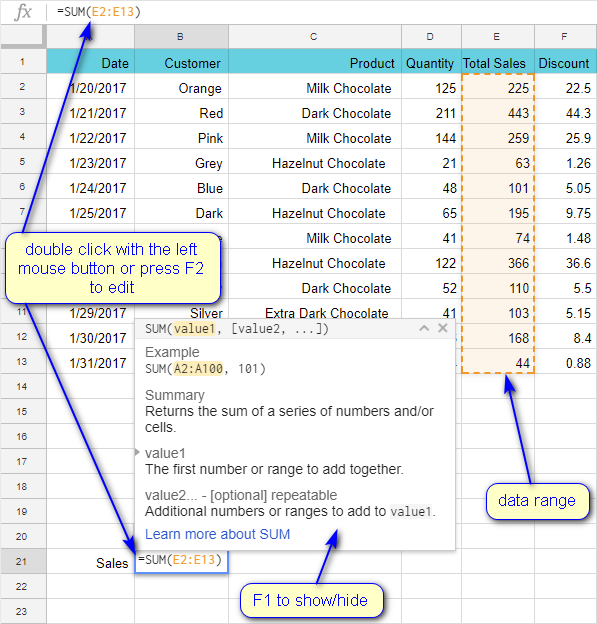
Tip. To hide only a function summary, press F1 on your keyboard. To turn off all formula hints, press Shift+F1. Use the same shortcuts to restore hints.
Reference other cells in Google Sheets formulas
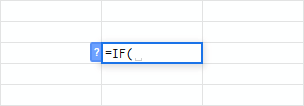
If you enter a formula and see a gray square bracket like on the next screenshot (it's called metrical tetraceme according to Unicode), it means the system is inviting you to enter a data range:
Select the range with your mouse, keyboard arrows, or type it manually. The arguments will be separated by commas:
=SUM(E2,E4,E8,E13)
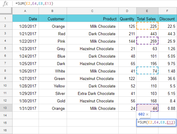
Tip. To select the range with the keyboard, use arrows to hop to the top leftmost cell of the range, press and hold Shift, and navigate to the right bottommost cell. The entire range will be highlighted and will appear in your formula as a reference.
Tip. To select non-adjacent ranges, keep Ctrl pressed while picking them with your mouse.
Reference data from other sheets
Google Sheets formulas can calculate data not only from the same sheet they are created in but also from other sheets. Let's say you want to multiply A4 from Sheet1 by D6 from Sheet2:
=Sheet1!A4*Sheet2!D6
Note. An exclamation mark separates a sheet name from a cell name.
To reference data ranges from multiple sheets, just list them using commas:
=SUM(Sheet1!E2:E13,Sheet2!B1:B5)
Tip. If a sheet name contains spaces, enclose the entire name to single quotation marks:
='Sheet 1'!A4*'Sheet 2'!D6
Edit references in existing formulas
So, your formula is created.
To edit it, either double-click the cell or click it once and press F2. You'll see all formula elements in different colors based on the type of value.
Use arrows on your keyboard to go to the reference you'd like to change. Once there, press F2. The range (or cell reference) will become underlined. It's a signal for you to set a new reference using one of the ways described earlier.
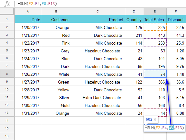
Press F2 again to replace the coordinates. Then work with arrows again to move your cursor to the next range or press Enter to leave editing mode and save the changes.
Nested functions
All functions use arguments for calculations. How do they work?
Example 1
Values written directly to the formula are used as arguments:
=SUM(40,50,55,20,10,88)
Example 2
Cell references and data ranges can also be arguments:
=SUM(A1,A2,B1,D2,D3)
=SUM(A1:A10)
But what if values you refer to haven't been calculated yet since they depend on other Google Sheets formulas? Can't you include them directly into your main function instead of cell-referencing them?
Yes, you can!
Example 3
Other functions can be used as arguments – they are called nested functions. Have a look at this screenshot:
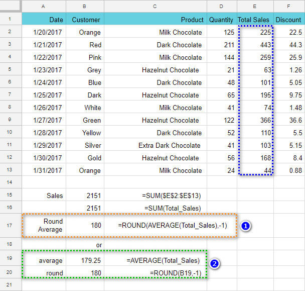
B19 calculates average sale amount, then B20 rounds it and returns the result.
However, B17 shows an alternative way of getting the same result with a nested function:
=ROUND(AVERAGE(Total_Sales),-1)
Simply replace cell reference with whatever lies directly in that cell: AVERAGE(Total_Sales). And now, first, it calculates average sale amount, then rounds the result.
This way you don't need to use two cells and your calculations are compact.
How to make Google Sheets show all formulas
By default, cells in Google Sheets return the results of calculations. You can see formulas only when editing them. But if you need to quickly check all formulas, there's one "view mode" that will help.
To make Google show all formulas and functions used in a spreadsheet, go to View > Show formulas in the menu.
Tip. To see the results back, just pick the same operation. You can switch between these views using Ctrl+' shortcut.
Remember my previous screenshot? Here's what it looks like with all the formulas:
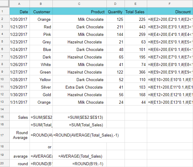
Tip. This mode is extremely helpful when you want to quickly check how your values are calculated and which ones are entered "by hand".
Copy formula over an entire column
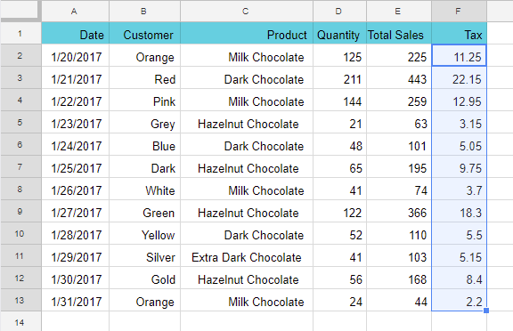
I have a table where I take note of all sales. I plan to add a column to calculate a 5% tax from each sale. I start with a formula in F2:
=E2*0.05
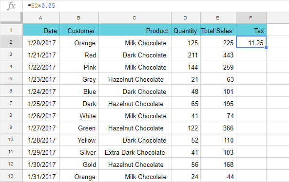
To fill all cells with the formula, one of the ways below will do.
Note. To copy the formula to other cells correctly, make sure you use absolute and relative cells references in a proper way.
Option 1
Make your cell with the formula active and hover the cursor over its bottom right corner (where a little square appears). Click the left mouse button and pull the formula as many rows below as needed:
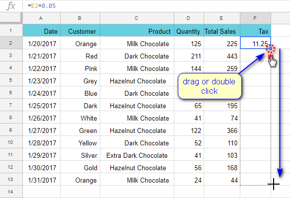
The formula will be copied over the entire column with the corresponding changes.
Tip. If your table is already packed with data, there's a much faster way. Just double-click that little square at the bottom right corner of the cell, and the entire column will be filled with the formulas automatically:
Option 2
Make the necessary cell active. Then press and hold Shift and use arrows on your keyboard to go the last cell of the range. Once picked, release Shift and press Ctrl+D. This will automatically copy the formula over.
Tip. To fill the row to the right of the cell, use the Ctrl+R shortcut instead.
Option 3
Copy the necessary formula to the Clipboard (Ctrl+C). Select the range you'd like to stuff and press Ctrl+V.
Option 4 – filling an entire column with the formula
If your source cell is in the very first row, select the entire column by clicking its header and press Ctrl+D.
If the source cell is not the first one, select it and copy to the Clipboard (Ctrl+C). Then press Ctrl+Shift+↓ (downward arrow) – this will highlight the entire column. Insert formula with Ctrl+V.
Note. Use Ctrl+Shift+→ (rightward arrow) if you need to fill the row.
In case you know any other useful tips on managing Google Sheets formulas, feel free to share them in comments below.
 by
by
One comment
Thank you! The F2 Solution was really helpful.