Did you know that when you merge Google sheets you can not only match & update records but also pull other related columns and even non-matching rows? Today I will show you how it's done with VLOOKUP, INDEX/MATCH, QUERY functions and the Merge Sheets add-on.
The last time I talked about merging Google sheets, I shared ways to match & update data. This time, we'll still update cells but will also pull other related columns and non-matching rows.
Here's my lookup table. I'm going to take all the necessary data from it today:
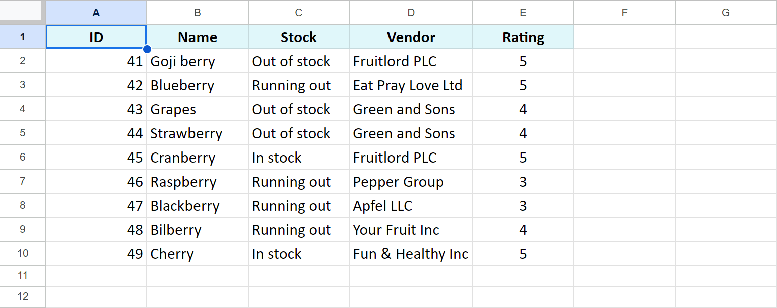
It's got bigger this time: it has two extra columns with vendor names and their ratings. I will update the Stock column with this info in another table and will also pull vendors. Well, maybe ratings as well :)
As usual, I will use a few functions and a special add-on for the job.
Merge Google sheets & add related columns using VLOOKUP
Remember Google Sheets VLOOKUP? I used it in my previous article to match data and update some cells.
If this function still scares you away, it's high time to face it and learn it once and for all because I'm going to use it today as well :)
Tip. If you're looking for a quick solution to save your time, go meet Merge Sheets right away.
Let's do a quick formula syntax recap:
- search_key is what you're looking for.
- range is where you're looking for.
- index is the number of the column to return the value from.
- [is_sorted] is completely optional and indicates whether the key column is sorted.
Tip. There's a whole tutorial devoted to Google Sheets VLOOKUP on our blog, feel free to have a look.
When I merged Google sheets and simply updated the data in the Stock column, I used this VLOOKUP formula:
=ArrayFormula(IFERROR(VLOOKUP($B$2:$B$10,Sheet1!$B$2:$D$10,2,FALSE),""))
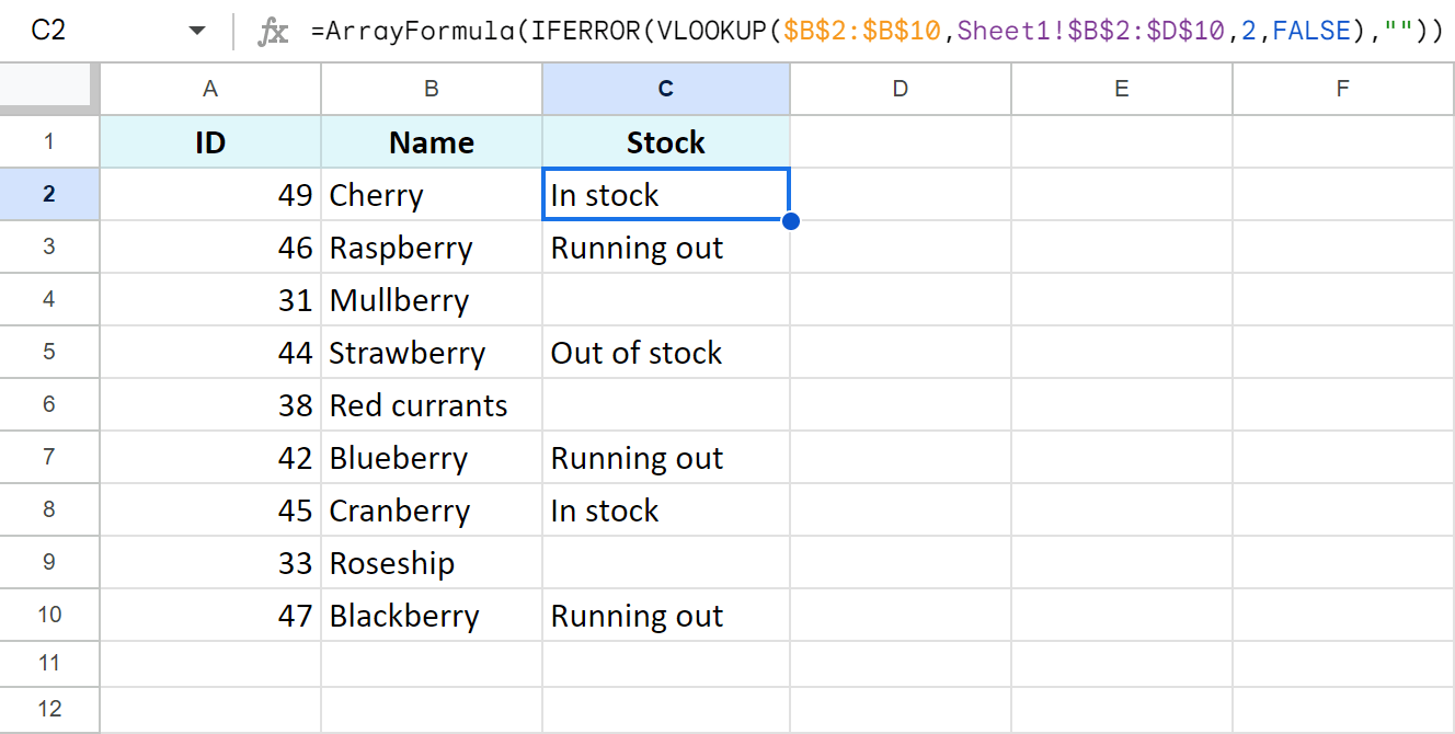
IFERROR made sure there were no errors in cells without matches and ARRAYFORMULA processed the entire column at once.
So what changes do I need to make to pull vendors as a new column from the lookup table as well?
Well, since it's the index that tells Google Sheets VLOOKUP what column it should take the data from, it's safe to say it's the one that needs tweaking.
The simplest way would be to just copy the formula into the neighboring column and increase its index by one (replace 2 with 3):
=ArrayFormula(IFERROR(VLOOKUP($B$2:$B$10,Sheet1!$B$2:$D$10,3,FALSE),""))
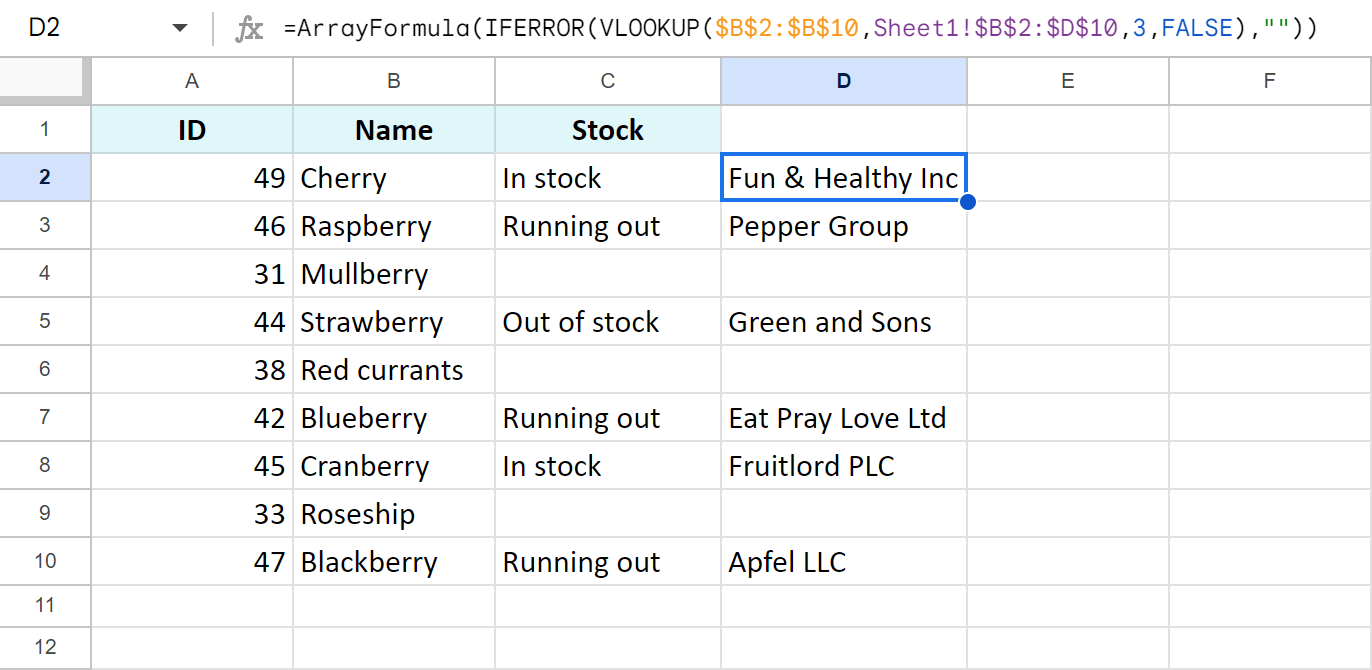
However, you'll need to insert the same formula with a different index as many times as many additional columns you'd like to get.
Fortunately, there's a better alternative. It involves creating arrays. Arrays let you combine all columns you'd like to pull in one index.
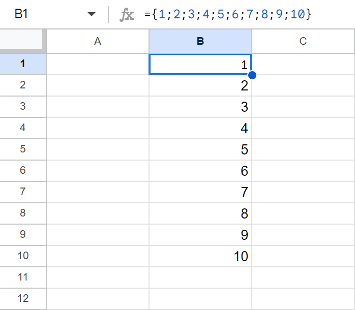
When you create an array in Google Sheets, you list values or cell/range references in brackets, e.g. ={1, 2, 3} or ={1; 2; 3}
The arrangement of these records in a sheet depends on the delimiter:
- If you use a semicolon, numbers will take up different rows within a column:
- If you use a comma, those numbers will appear in separate columns in a row:

The latter is exactly what you need to do in the Google Sheets VLOOKUP index argument.
Since I merge Google sheets, update the 2nd column and pull the 3rd one, I need to create an array with these columns: {2, 3}:
=ArrayFormula(IFERROR(VLOOKUP($B$2:$B$10,Sheet1!$B$2:$D$10,{2,3},FALSE),""))
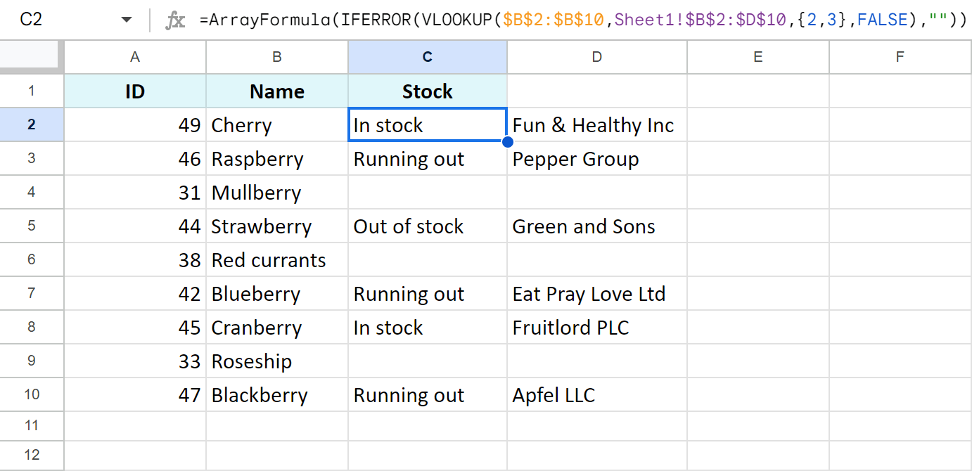
This way, one Google Sheets VLOOKUP formula matches names, updates stock info and adds related vendors into an empty adjacent column.
Match & merge sheets and add columns with INDEX MATCH
Next up is INDEX MATCH. These two functions together compete with VLOOKUP as they bypass its limitations when merging Google sheets.
Tip. Get to know INDEX MATCH for Google Sheets in this tutorial.
Let me start by reminding you of the formula that simply merges one column based on the matches:
=IFERROR(INDEX(Sheet1!$C$1:$C$10,MATCH(B2,Sheet1!$B$1:$B$10,0)),"")
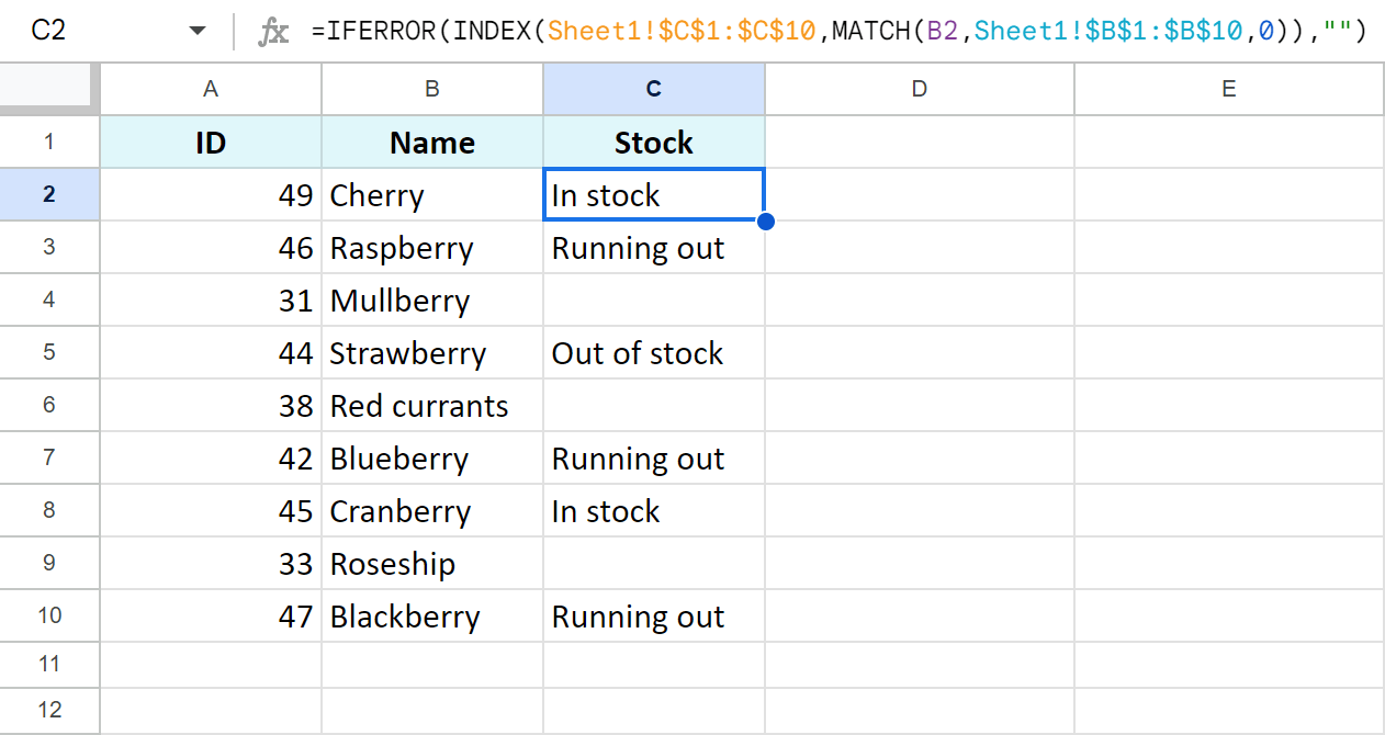
In this formula, Sheet1!$C$1:$C$10 is a column with the values you need whenever Sheet1!$B$1:$B$10 meets the same value as in B2 in the current table.
With these points in mind, it is Sheet1!$C$1:$C$10 that you need to change in order to not just merge tables and update cells but also add columns.
Unlike Google Sheets VLOOKUP, nothing fancy here. You just enter the range with all those required columns: the one to update and others to add. In my case, it'll be Sheet1!$C$1:$D$10:
=IFERROR(INDEX(Sheet1!$C$1:$D$10,MATCH(B2,Sheet1!$B$1:$B$10,0)),"")
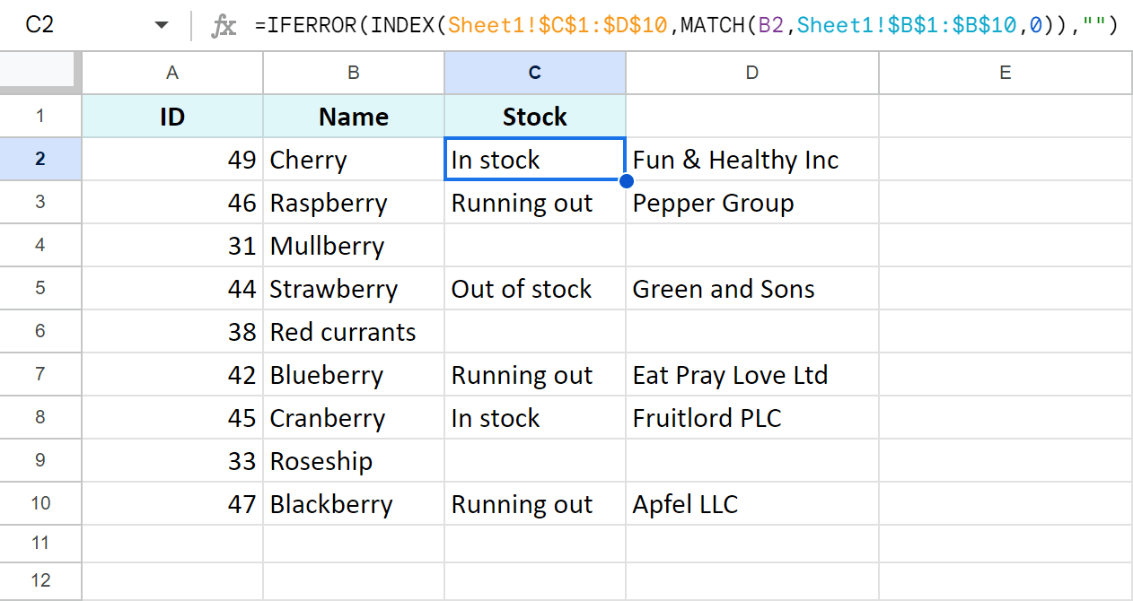
Or I can expand the range to E10 to add 2 columns, not just one:
=IFERROR(INDEX(Sheet1!$C$1:$E$10,MATCH(B2,Sheet1!$B$1:$B$10,0)),"")
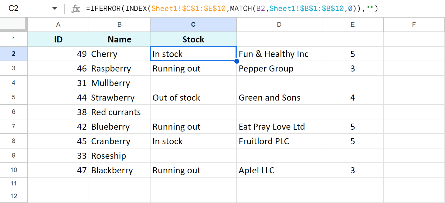
Note. Those extra records always fall into the neighboring columns. If those columns will have some other values, the formula won't overwrite them. It will give you a #REF error with a corresponding hint:
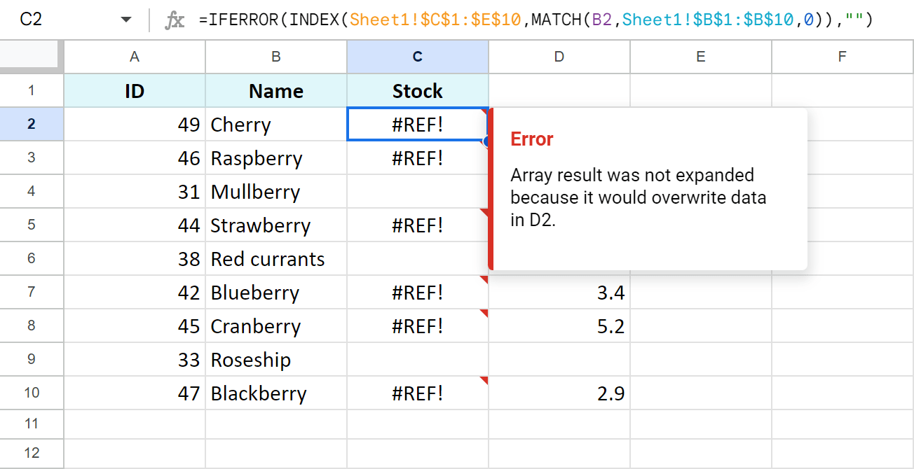
Once you clear those cells or add new columns to the left of them, the formula results will appear.
Merge Google sheets, update cells & add related columns — all using QUERY
QUERY is one of the most powerful functions in Google spreadsheets. So it's no surprise I'm going to use it today to merge some Google sheets, update cells and add extra columns at the same time.
This function differs from others because one of its arguments uses a command language.
Tip. If you're wondering how to use the Google Sheets QUERY function, visit this blog post.
Let's recall the formula that updates cells first:
=IFERROR(QUERY(Sheet1!$A$2:$C$10,"select C where B='"&Sheet4!$B2:$B$10&"'"),"")
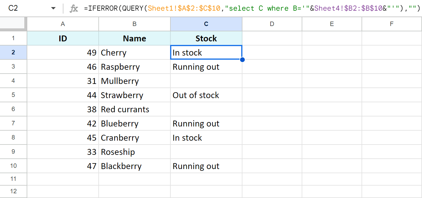
Here QUERY looks at the table with the required data in Sheet1, matches cells in column B with my current new table, and merges these sheets: pulls data from column C for every match. IFERROR keeps the result error-free.
To add extra columns for those matches, you need to make 2 small changes to this formula:
- list all must-have columns for the select command:
…select C,D,E… - expand the range to look accordingly:
…QUERY(Sheet1!$A$2:$E$10,…
Here's a full formula:
=IFERROR(QUERY(Sheet1!$A$2:$E$10,"select C,D,E where B='"&Sheet4!$B2:$B$10&"'"),"")
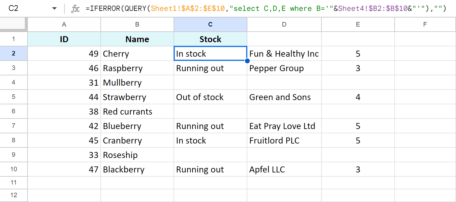
It updates the stock column and pulls 2 extra columns from the lookup table to this main table.
How to add non-matching rows using FILTER + VLOOKUP
Imagine this: you merge Google sheets, update old info with the new one, and get new columns with extra related values.
What else could you do to have a full picture of the records at hand?
Perhaps adding non-matching rows to the end of your table? This way, you'll have all values in one place: not only matches with the updated related info but also non-matches as well to make them count.
I was pleasantly surprised that Google Sheets VLOOKUP knows how to do that. When used together with the FILTER function, it merges Google sheets and adds non-matching rows as well.
Tip. In the end, I will also show how one add-on does the same with a single checkbox.
Google Sheets FILTER arguments are pretty clear:
- range is the data you want to filter.
- condition1 is a column or a row with a filtering criterion.
- criteria2, criteria3, etc. are completely optional. Use them when you need to use several criteria.
Tip. You will learn more about the Google Sheets FILTER function in this blog post.
So how do these two functions get along together and merge Google sheets? Well, FILTER returns the data based on the filtering criteria created by VLOOKUP.
Look at this formula:
=FILTER(Sheet1!$A$2:$E$10,ISERROR(VLOOKUP(Sheet1!$B$2:$B$10,$B$2:$C$10,2,FALSE)=1))
It scans Google tables for matches and pulls non-matching rows from one table to the other:
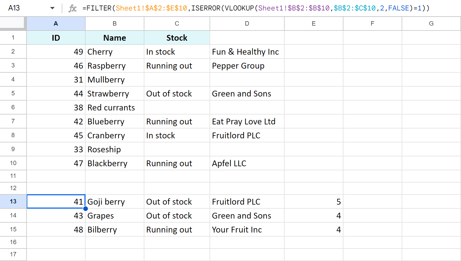
Let me explain how it works:
- FILTER goes to the lookup sheet (a table with all the data — Sheet1!$A$2:$E$10) and uses VLOOKUP to get the correct rows.
- VLOOKUP takes the names of the items from column B on that lookup sheet and matches them with the names from my current table. If there's no match, VLOOKUP says there's an error.
- ISERROR marks each such error with 1, telling FILTER to take this row into another sheet.
As a result, the formula pulls 3 additional rows for those berries that don't occur in my main table.
It's not that complicated once you play around with this method a bit :)
But if you don't want to spend your time on this, there's a better and quicker way — without a single function and formula.
Formula-free way to match & merge data — Merge Sheets add-on
Merge Sheets add-on encompasses all 3 possibilities when merging Google sheets:
- it updates related cells based on the matches
- adds new columns for those matches
- inserts rows with non-matching records
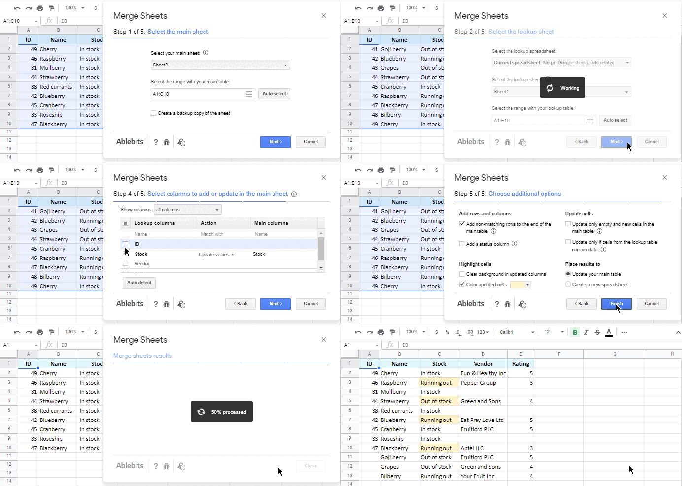
To avoid any confusion, the process is divided into 5 simple steps:
- The first two are where you select your tables even if they are in different spreadsheets.
- On the 3d, you are to choose key column(s) that should be checked for matches.
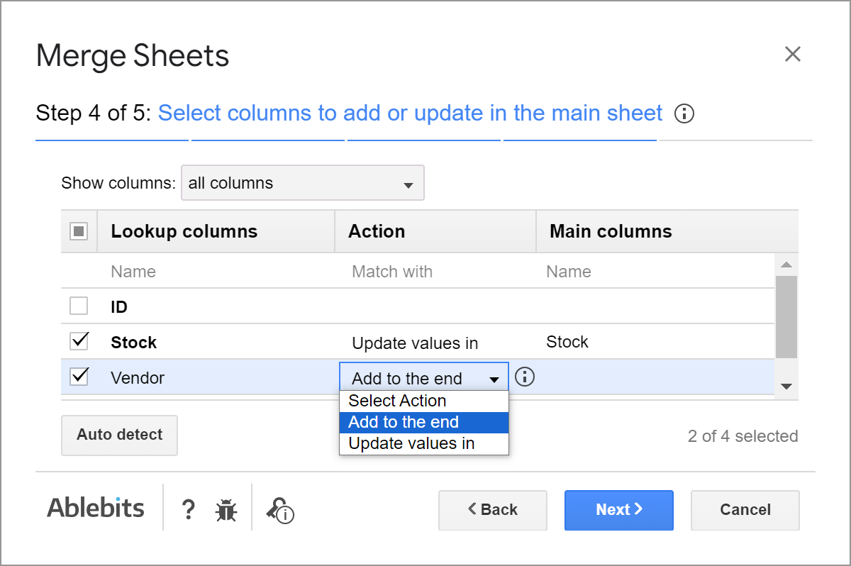
- The 4th step lets you set the columns to update with new records or add from one sheet to another:
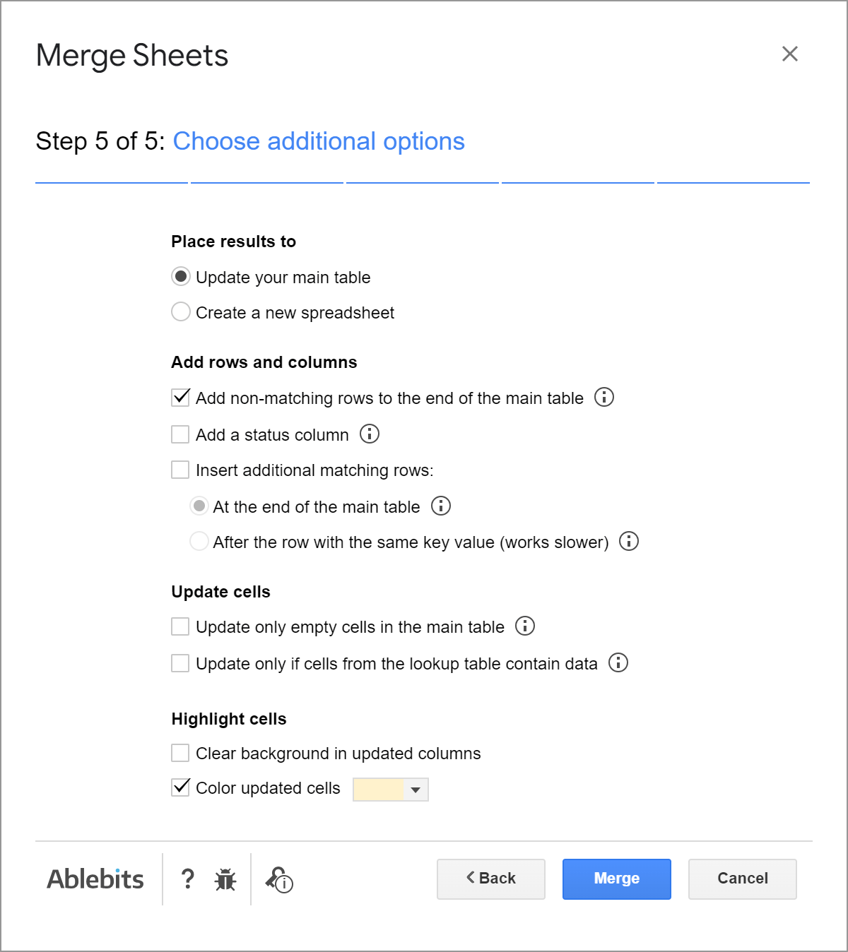
- Finally, the 5th step has that checkbox that will make all non-matching rows appear at the end of your current table:
It took a few seconds till I could see the result:
Video: How to merge Google sheets, update cells, add extra columns and rows
This 3-minute demo video will help you make up your mind regarding trying Merge Sheets out :)
Install Merge Sheets from the Google Sheets store and you'll see that it processes bigger tables just as fast. Thanks to Merge Sheets, you'll have more time for important matters.
Spreadsheet with formula examples
Merge Google sheets, add related columns & non-matching rows - formula examples (make a copy of this spreadsheet)
 by
by
11 comments
Dear Natalia Sharashova,
I need to pull the data from main sheet to dash board sheet based on if I select specific department and specific work type but in main sheet departments are presented in A1 to Z1 column and work type are presented in B:B column i used filter function array formula etc but every formula showing some error
Hello Manikandan Selvaraj,
For me to be able to assist you, please share a small sample spreadsheet with us (support@apps4gs.com) with (1) a copy of your source data (2) the result you expect to get. The result sheet is of great importance as it gives us a better understanding than any text description.
I kindly ask you to shorten the tables to 10-20 rows.
Note. We keep that Google account for file sharing only and don't monitor its Inbox. Do not email there. Once you share the file, just confirm by replying to this comment.
I'll look into your task and try to help.
Dear Natalia Sharashova,
As per your needed, I ill share source data file along with expect result to support@apps4gs.com
file shared
Thank you for sharing the file, Manikandan Selvaraj.
Unfortunately, the task you've outlined is too complex and falls outside the scope of the support we provide. I wish I could help you more.
K can you suggest any ideas to make it for example which formula can I use like that
INDEX MATCH or QUERY are often used to pull data based on different criteria. But you may need to restructure the table to use these functions effectively.
I've been searching through your guides and learned some things about queries. I am trying to combine 3 lists into one, and only show the most recent instance of each.
I've created a query formula that combines the 3 lists well:
=QUERY({'Cheevo Calendar'!A3:D;'Cheevo Calendar'!F3:I;'Cheevo Calendar'!R3:U}, "SELECT Col2, Col1, Col3, Col4 WHERE Col2 ''ORDER BY Col1 ASC", 0)
And I did a SORTN formula to filter for my desired results, but it sorted by planet, not most recent instance of each:
=sortn(sort(A4:D,2,0),9^9, 2,1,1)
Is there a way to achieve these results in one formula?
I would also like to show which source each row came from if possible, but that's just a bonus.
Here's a sample of my spreadsheet:
https://docs.google.com/spreadsheets/d/1NTXBpcFRQa_6wDFWNoXdG48gNJ_bdA74dqCPUGYh0qs/edit?usp=sharing
Thanks!
Hello Brenna,
I'm afraid there's no one easy formula for the task. So I'd suggest sticking to several steps with several formulas.
You can return column names with your first QUERY:
=ARRAYFORMULA(QUERY({'Cheevo Calendar'!A3:D,TEXT('Cheevo Calendar'!A3:D,"")&'Cheevo Calendar'!$A$1;'Cheevo Calendar'!F3:I,TEXT('Cheevo Calendar'!F3:I,"")&'Cheevo Calendar'!$F$1;'Cheevo Calendar'!K3:N,TEXT('Cheevo Calendar'!K3:N,"")&'Cheevo Calendar'!$K$1}, "SELECT Col2, Col1, Col3, Col4,Col5 WHERE Col2 <> ''ORDER BY Col1 ASC", 0))
The next formula will use SORTN & sort data by dates:
=SORTN(SORT(A3:D80, 2, 0), ROWS(A3:A80), 2, 1, 1)
Hope these will help!
I dont see any merges, why do you mention that
Hello Raj,
The first image (right under the TOC) is my lookup table. All formulas in the blog post match records between that lookup table and the tables the formulas are used in. This is the merge. Two tables are being matched and merged.
If you'd like to read about the simple combining of the tables, perhaps, this blog post is what you're looking for.