Every once in a while each Google Sheets user faces the inevitable: combining several sheets into one. Copy-pasting is tedious and time-consuming, so there has to be another way. And you're right — there are several ways, in fact. So get your tables ready and follow the steps from this article.
All the ways I describe can be used to process large tables. But to keep this guide as clear as possible, I'll keep my tables short and am going to cut down to a couple of sheets.
Reference cells in Google Sheets to pull data from another tab
The easiest way comes first. You can pull entire tables to one file by referencing cells with data from other sheets.
Note. This will do if you need to merge two or more sheets within one Google spreadsheet. To merge multiple Google spreadsheets (files) into one, jump right to the next method.
So, my data is scattered all over different sheets: June, July, August. I'd like to pull data from July and August into June to have one table as a result:
- Find the first blank cell right after your table (the June sheet for me) and place the cursor there.
- Enter your first cell reference. The first table I want to retrieve starts from A2 in the July sheet. So I put:
=July!A2Note. If there are spaces in your sheet name, you must wrap it in single quotes like this:
='July 2022'!A2This immediately replicates whatever lies in that cell:

Note. Use relative cell reference so it changes itself when copied to other cells. Otherwise, it will return incorrect data.
- Make sure the cell with the reference is selected and click on that little blue square at its bottom right corner. The mouse cursor will turn into a big black plus sign. Keep the mouse pressed and drag the cursor to as many columns to the right as you need to fill them with new records:

- Select this entire new row, click that little blue square once again, hold and drag your mouse down — this time to fill entire rows with cell references and bring new data from another sheet:
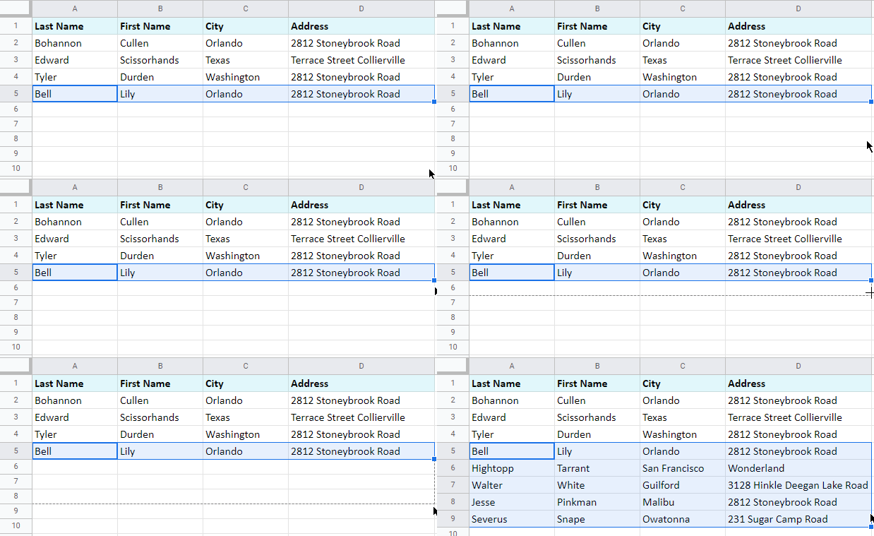
Though this is probably the first way you may think of to pull data from another tab, it's not the most elegant and quick. Luckily, Google prepared other instruments specially for this purpose.
Copy the tabs into one spreadsheet
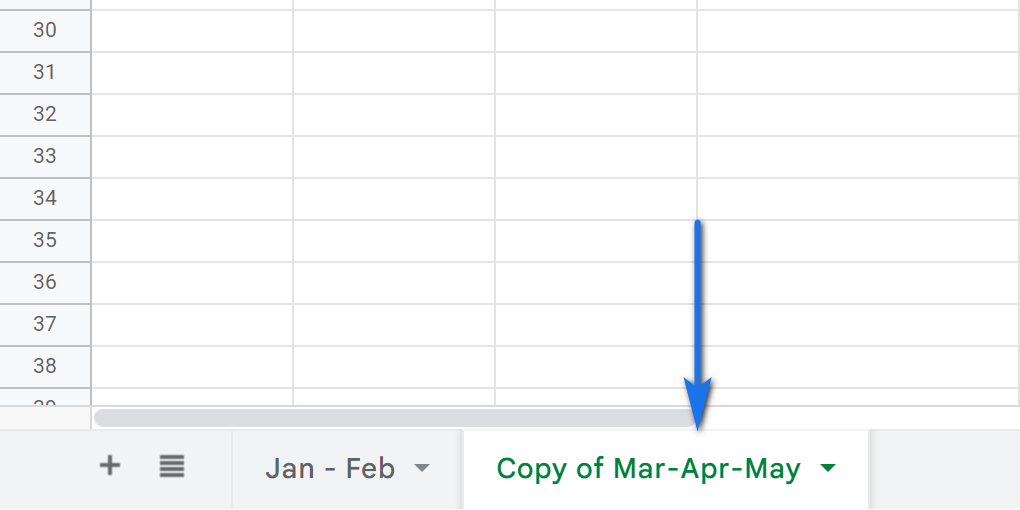
One of the standard ways is to copy the tabs of interest into the destination spreadsheet:
- Open the file that contains the sheet(s) you want to transfer.
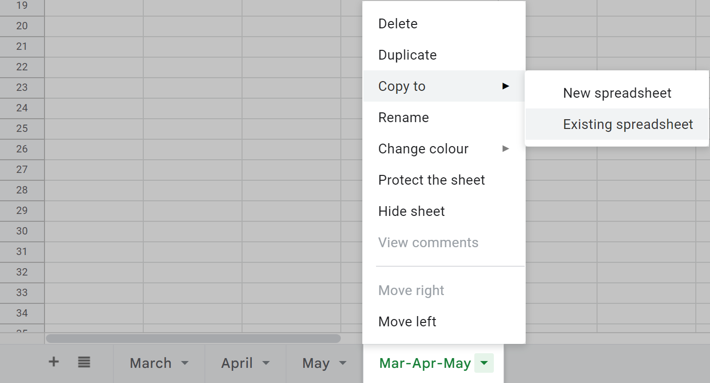
- Right-click the first tab you need to export and choose Copy to > Existing spreadsheet:
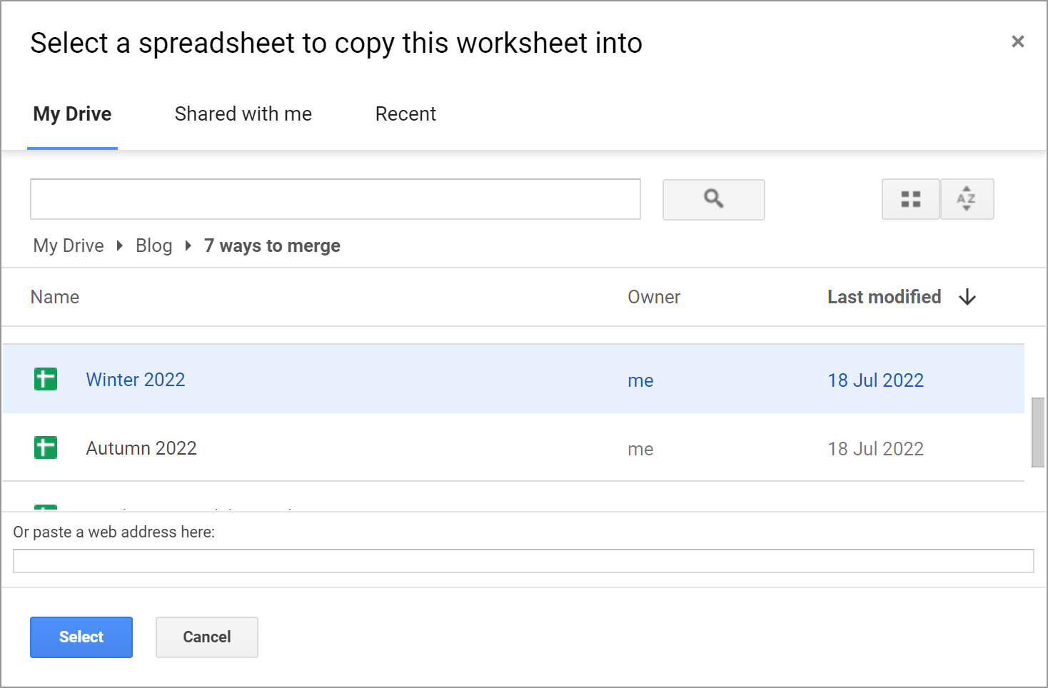
- The next thing you'll see is the pop-up window inviting you to select the spreadsheet. Browse for it, click on it to highlight it, and press Select when you're ready:
- Once the sheet is copied, you'll get a corresponding confirmation message:

- You can either hit OK and continue with the current sheet or follow the link called Open spreadsheet. It will instantly get you to another spreadsheet with the first sheet already there:
Export/import sheets
Another way to import data from multiple Google Sheets is to export each sheet first, and then import them all to a necessary file:
- Open the spreadsheet that contains the sheet you'd like to pull the data from.
- Make the sheet of interest active by selecting it.
- Go to File > Download > Comma-separated values (.csv):
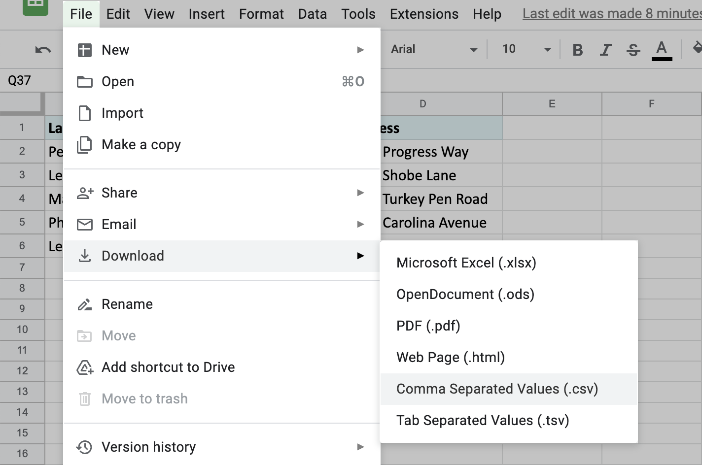
The file will be downloaded to your computer.
- Then open another spreadsheet — the one you'd like to add the sheet to.
- This time, pick File > Import from the menu and go to the Upload tab in the Import file window:
- Hit Select a file from your device and find the sheet you've downloaded just now.
- Once the file is uploaded, you'll see a window with additional options for importing the sheet. To add the contents of that another sheet after your existing table, pick Append to current sheet:
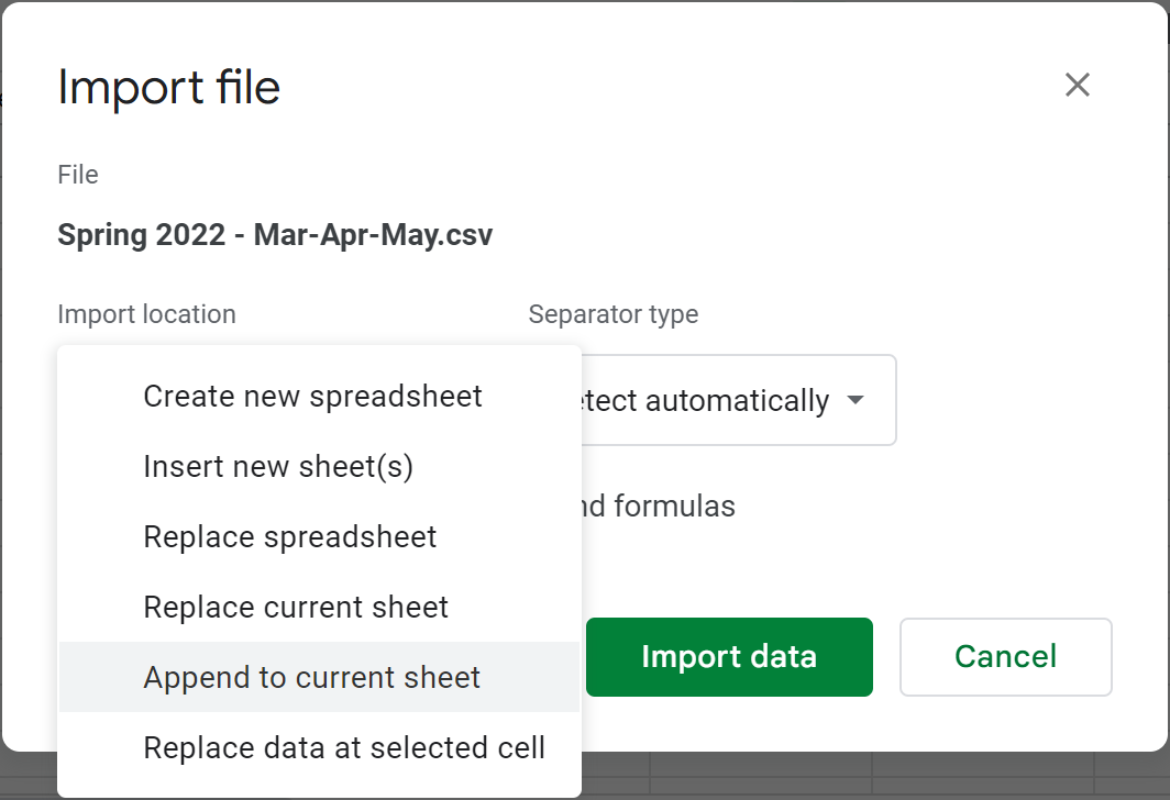
Tip. Among other settings, feel free to specify the separator and convert text to numbers, dates, and formulas.
- As a result, you'll get two sheets merged — one table under another:
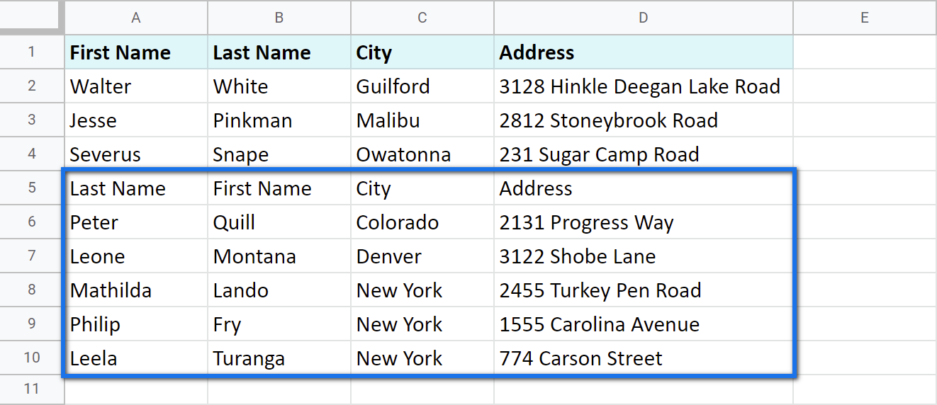
But since it is a .csv file you need to import, the second table remains formatted in a standard way. You will have to spend some time formatting it as you need.

Google Sheets functions to combine data from multiple spreadsheets
Of course, it wouldn't be Google if it didn't have functions to merge data in Google Sheets.
IMPORTRANGE to import data from multiple Google sheets
As the name of the function suggests, IMPORTRANGE imports data from multiple Google spreadsheets into one sheet.
Tip. The function helps Google Sheets pull data from another document as well as from other tabs from the same file.
Here's what the function requires:
- spreadsheet_url is nothing else than the link to the spreadsheet from where you need to pull the data. It must always be put between double-quotes.
- range_string stands for those cells specifically that you need to bring to your current sheet.
And here's the pattern I follow to import data from multiple Google Sheets using IMPORTRANGE:
- Open the spreadsheet from which you want to pull the data.
Note. Make sure you have at least viewing access to that file.
- Click the browser URL bar and copy the link to this file right till the hash sign (#):
- Return to the spreadsheet where you want to add the info to, enter the IMPORTRANGE to where the borrowed table should appear, and insert the link as the first argument. Then separate it from the next part with a comma:
- For the second part of the formula, type in the name of the sheet and the exact range that you want to pull. Confirm by pressing Enter.
Note. Wrap the second argument in double quotes as well:
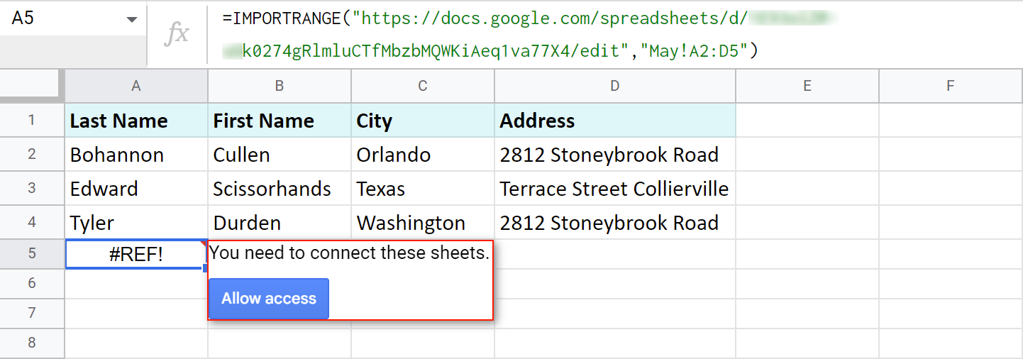
=IMPORTRANGE("https://docs.google.com/spreadsheets/d/XYZk0274gRlmluCTfMbzbMQWKiAeq1va77X4/edit","May!A2:D5") - Though the formula looks ready now, it will return the #REF error from the start. That's because the first time you try to pull data from some spreadsheet, IMPORTRANGE will ask for access to it. Once the permission is granted, you will easily import records from other sheets of that file.
Click the cell with the error and press that blue Allow access prompt:
- Once the formula connects to that other sheet, it will import data from there:
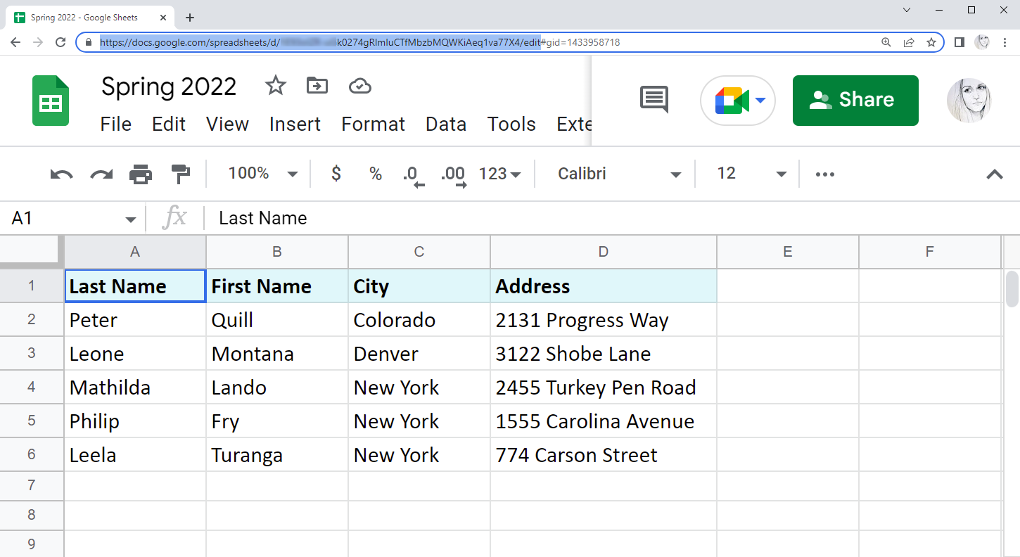
Note. You'll need this URL even if you're going to combine sheets from the same file.
Tip. Though Google says the function requires the whole URL, you can easily get by with a key — a part of the URL between /d/ and /edit:
...google.com/spreadsheets/d/XYZk0274gRlmluCTfMbzbMQWKiAeq1va77X4/edit

Note. Remember, the link should be surrounded by double quotes.
Note. By allowing access, you let the Sheets know you don't mind any existing or potential collaborators on this spreadsheet accessing data from another file.
Note. IMPORTRANGE doesn't pull the formatting of the cells, only values. You will need to apply formatting manually afterwards.
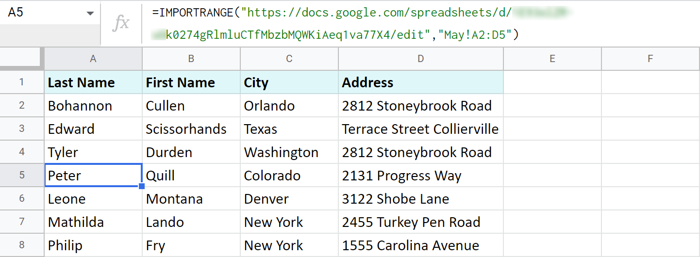
Tip. If the tables are rather big, just allow some time for the formula to pull all records.
Note. The records returned by the function will be updated automatically if you change them in the original file.
Google Sheets QUERY to import ranges from multiple sheets
And thus, without haste, we've come to the QUERY function once again. :) It is so versatile that can be used in Google spreadsheets to combine data from multiple sheets (within the same file) as well.
So, I want to merge three different Google sheets (from one file): Winter 2022, Spring 2022, and Summer 2022. They contain the names of all employees who became best in their jobs in different months.
I go to the first sheet — Winter 2022 — and add my QUERY right under the existing table:
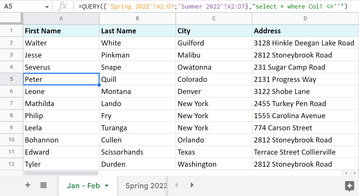
=QUERY({'Spring 2022'!A2:D7;'Summer 2022'!A2:D7},"select * where Col1 <>''")
Let's see what it all means:
- {'Spring 2022'!A2:D7;'Summer 2022'!A2:D7} — are all the sheets and ranges I need to import.
Note. The sheets should be written in between the curly brackets. If their names contain spaces, use single quotes to list the names.
Tip. Separate the ranges with a semicolon to pull data from different tabs one under another. Use commas instead to have them imported side by side.
Tip. Feel free to use such infinite ranges as A2:D.
- select * where Col1 <>'' — I tell the formula to import all records (select *) only if cells in the first column of the tables (where Col1) are not blank (<>''). I use a pair of single quotes to indicate the non-blanks.
Note. I use <>'' because my column contains text. If your column contains other data type (e.g. date or time, etc.), you need to use is not null instead: "select * where Col1 is not null"
As a result, two tables from other sheets have been consolidated into one sheet one under another:
Tip. If you'd like to use Google Sheets QUERY to import ranges from multiple separate spreadsheets (files), you will have to implement IMPORTRANGE. Here's a formula to pull your data from other documents:
=QUERY({IMPORTRANGE("XYZk0274gRlmluCTfMbzbMQWKiAeq1va77X4","Mar-Apr-May!A2:D6");IMPORTRANGE("XYZahJZHSlhMGLSW_xA6ZBqNmt1I0ADo4N4M","Jun-Jul-Aug!A2:D4")},"select * where Col1<>''")
Tip. I use the keys from URLs rather than entire links in this long-enough formula. If you're not sure what that is, please read here.
Tip. You can also use QUERY to merge two Google sheets, update cells, add related columns & non-matching rows. Check this out in this blog post.
3 quickest ways to merge multiple Google sheets
If standard ways of Google spreadsheets to combine data from multiple sheets seem dull, and the functions scare you off, there's an easier approach.
Combine Sheets add-on
This first special add-on — Combine Sheets — was designed with a single purpose: import data from multiple Google sheets.
It's clever enough to recognize the same columns in different sheets and bring data together accordingly if you need.

All you are to do is:
- Select sheets or entire spreadsheets to merge and specify the ranges if necessary. A quick search across your Drive makes this even faster.
- Choose how to pull the data:
- as a formula. Mark the checkbox called Use a formula to combine sheets if you want to have a master sheet that will dynamically change based on your original contents.
Although you won't be able to edit the resulting table, its formula will be always linked to the source sheets: edit a cell or add/remove entire rows there, and the master sheet will be altered accordingly.
- as values. If editing the resulting table manually is more important, ignore the above option and all data will be combined as values.
Extra options are here for fine-tuning:
- join records from the same columns into one column
- keep the formatting
- add a blank line between different ranges to notice them right away
- as a formula. Mark the checkbox called Use a formula to combine sheets if you want to have a master sheet that will dynamically change based on your original contents.
- Decide where to place the merged table: new spreadsheet, new sheet, or in a location of your choice.
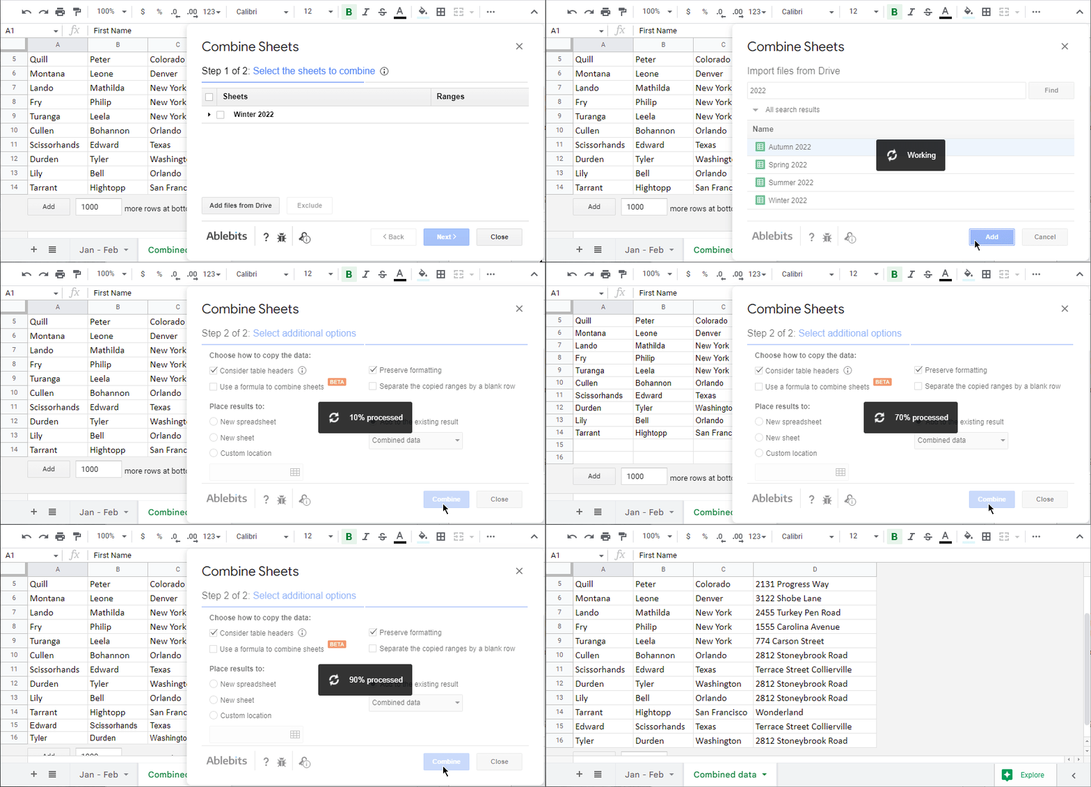
Here's a quick demonstration of how I combined my three small tables with the add-on:
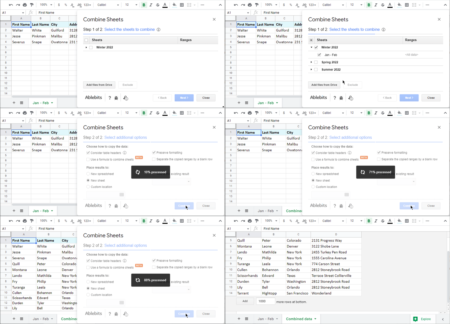
Of course, your tables can be much bigger and you can merge lots of different sheets as long as the resulting file doesn't exceed the 10M cell-limit.
One of the options this add-on offers is to add more sheets to your previously combined data. In this case on step 1, you need to pick not only the data to combine but also the existing result. Here's how it looks:
Video: How to combine multiple Google sheets into one
Check out the help page for Combine Sheets or watch this 3,5-minute tutorial:
Consolidate Sheets add-on
Consolidate Sheets is another handy tool among our add-ons. Its main difference from the aforementioned tool is the ability to add up data in columns in Google Sheets (or rows, or single cells, for that matter).
Consolidate Sheets also recognizes common headers in all the Google sheets to join, even if they are in the leftmost column and/or the first row. There's always an option to merge Google sheets and calculate cells based on their place in the tables.
Let me break it down into steps for you as well:
- Select sheets to consolidate. Import more files from Drive if necessary straight from the add-on.
- Pick the function to consolidate in Google Sheets.
- Choose the way to add up cells in Google Sheets: by labels (header labels, left column labels, or both) or position.
- Decide where to place the consolidated data: new spreadsheet, new sheet, or any specific location within the opened file.
Here's how this process looks:
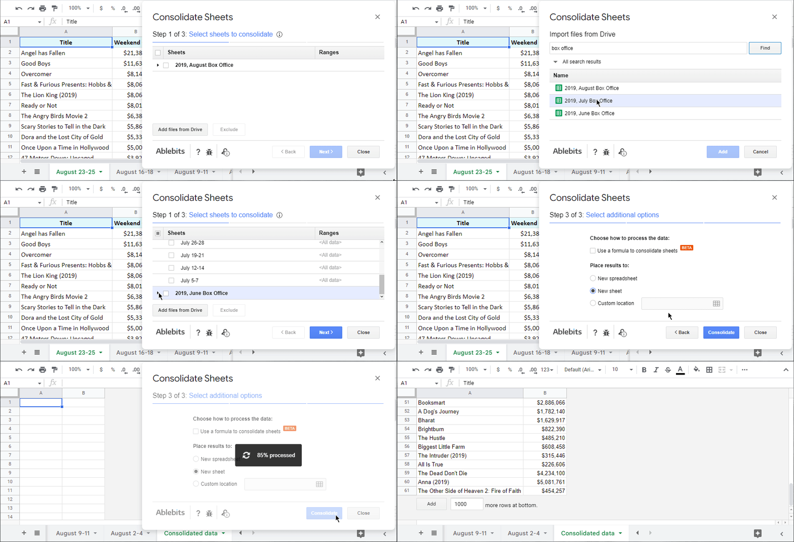
There's also an option to consolidate all your sheets using a formula. This way your result will change in sync with the values in the source sheets:
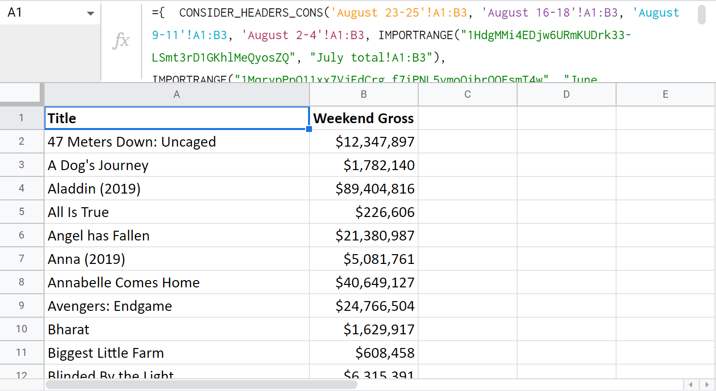
Note. There are some peculiarities you need to know about how the formula works. For example, if you consolidate from multiple different files, there will be an extra step to connect the sheets for the IMPORTRANGE in use. Please visit the instructional page for Consolidate Sheets for these and other details.
Video: How to consolidate multiple Google sheets into one
Here's a 4-minute demo-video about the add-on work:
I truly encourage you try this add-on. You'll see for yourself how much extra time you'll have after incorporating this tool to your daily work.
Merge Sheets add-on
There's one more add-on worth mentioning — Merge Sheets. It matches records from the same column in several sheets/documents and then pulls related data from the lookup sheets/documents into the main one. Hence, you always have an up-to-date spreadsheet at hand.
There are 5 straightforward steps:
- Select your main sheet.
- Select your lookup sheet (even if it's in another spreadsheet).
- Choose columns where matching records may occur.
- Tick of the columns with records to update.
- Tweak any additional options that will help you merge two sheets and achieve the best result possible.
You can even save the settings into reusable scenarios and run them later in a click.
Video: How to merge Google sheets
I know a picture is worth a thousand words, so here's a 3-minute video tutorial on Merge Sheets for you:
Ready to try it for yourself?
or visit this help page for details about each step and setting.
On this note, I'm going to finish this article. Hope these ways of pulling data from multiple different sheets into one will be of use. As always, looking forward to your comments!
 by
by 
220 comments
I was able to figure it out with this:
=QUERY({Kindergarten!A2:E;'1st'!A2:E;'2nd'!A2:E;'3rd'!A2:E;'4th'!A2:E;'5th'!A2:E;'6th'!A2:E;'7th'!A2:E;'8th'!A2:E;'9th'!A2:E;'10th'!A2:E;'11th'!A2:E;'12th'!A2:E},"select * where Col1>=date '"&TEXT(TODAY(),"YYYY-MM-DD")&"' ",1)
Thank you so much for your help!
My next task is to take this queried data and put it in time order. Right now it is in order of the sheets brought in.
This formula takes not only records for 'today's date' but all next days as well since you use the >= condition. But I'm glad if it works for you.
As for ordering data, add the 'order by' clause:
=QUERY({Kindergarten!A2:E;'1st'!A2:E;'2nd'!A2:E;'3rd'!A2:E;'4th'!A2:E;'5th'!A2:E;'6th'!A2:E;'7th'!A2:E;'8th'!A2:E;'9th'!A2:E;'10th'!A2:E;'11th'!A2:E;'12th'!A2:E},"select * where Col1>=date '"&TEXT(TODAY(),"YYYY-MM-DD")&"' order by Col1 ",1)
This what what my timestamp looks like: Thu, Jul 29, 2021 @ 10:19 AM
Basically I have created a query based on information of students checking in and out of school. Students check using a google form which gives me a time stamp when converted to google sheets. Then it is filtered out into differnet tabs where columns are deleted for the each teacher based upon a grade. I want the query an office report that pulls over from each teacher tab only today's students and not those who checked in and out yesterday. How do I query based on that time stamp to report only students who enter and exit my room today? My data columns are A (Timestamp), B In or Out), C (Grade), D (Name), E (reason). I need this to automatically filter/query everday.
My current formula looks like this:
=QUERY({Kindergarten!A2:E;'1st'!A2:E;'2nd'!A2:E;'3rd'!A2:E;'4th'!A2:E;'5th'!A2:E;'6th'!A2:E;'7th'!A2:E;'8th'!A2:E;'9th'!A2:E;'10th'!A2:E;'11th'!A2:E;'12th'!A2:E},"select * where Col1 is not Null")
This works, but it pulls all data over. I am pretty sure that I need the change the area after "select", but not sure what to change it to to only pull over those with a timestamp for today.
You're right, it's the part after 'select *' that needs changes. Try this one:
=QUERY({Kindergarten!A2:E;'1st'!A2:E;'2nd'!A2:E;'3rd'!A2:E;'4th'!A2:E;'5th'!A2:E;'6th'!A2:E;'7th'!A2:E;'8th'!A2:E;'9th'!A2:E;'10th'!A2:E;'11th'!A2:E;'12th'!A2:E},"select * where (Col1 >= datetime '"&TEXT(TODAY(),"yyyy-mm-dd HH:mm:ss")&"' and C <= datetime '"&TEXT(TODAY()+0.99999,"yyyy-mm-dd HH:mm:ss")&"')", 1)
I am getting a value error message stating: Unable to parse query string for Function QUERY parameter 2: NO_COLUMN: C
Should: and C <= datetime '"&TEXT(TODAY()+0.99999,"yyyy-mm-dd HH:mm:ss")&"')", 1) be 'A'?
I was able to figure it out with this:
=QUERY({Kindergarten!A2:E;'1st'!A2:E;'2nd'!A2:E;'3rd'!A2:E;'4th'!A2:E;'5th'!A2:E;'6th'!A2:E;'7th'!A2:E;'8th'!A2:E;'9th'!A2:E;'10th'!A2:E;'11th'!A2:E;'12th'!A2:E},"select * where Col1>=date '"&TEXT(TODAY(),"YYYY-MM-DD")&"' ",1)
Thank you so much for your help!
My next task is to take this queried data and put it in time order. Right now it is in order of the sheets brought in.
Yes, my apologies, there should be your column with dates instead of C: 'A' or even 'Col1'
I am trying to pull in data from13 diferent tabs from one worksheet to another. The data on these tabs will change daily and it includes an automatic timestamp. The data I want bring over from these tabs is only when the timestamp is for today. How do I go about doing that?
Hello Shawna,
Since you need to include the date as a condition, you should use formulas for your task.
You can either build a QUERY formula with the 'where' clause to pull only when there's a certain date in a certain column, or use our Combine Sheets to combine data with a formula first and then edit this formula by adding the same condition for column+date with the 'where' clause.
thanks, but if this date changes everyday how can it be done without editing the query formula everyday?
Can you specify how the timestamps look exactly? Maybe there are some date/time formulas you'll be able to incorporate.
Hey there,
I am having trouble wrapping my head around this so hopefully you can help.
I currently have a "master" project sheet that takes data from each sheet in the workbook and combines it adding to the list each time a new sheet is duplicated (using a template sheet)
1. Duplicate the "customer project data sheet" which would hold info such as expenses job costing, time on job etc.
2. Within this sheet I will grab totals and have all of the details essentially for that one project.
3. Now the trouble I am having is, if I have a template that talks back to the master sheet correctly I need it to continue to take the "totals" of the data in each customer project data sheet and enter it in the correct cells on the master sheet automatically as long as the data is entered in the correct locations on the template "customer project data sheet" (which would get named upon duplication with the client name)
So is it possible for gSheets to know that
1. After I duplicate a template it will know that all cells from the "template customer data" being pushed to master will do the same on each template sheet each time it is duplicated and data is entered in the cells requested within that sheet?
2. Then possibly easier fix, if the above can happen how do we get it to essentially continue adding the data but not sending it to the exact same cell, but rather continue to go down adding the data in a list form. Which then on the master project sheet I will be able to see the overall details, totals etc?
Overall I will have: Master Project Sheet (all needed data from customer sheets routed to this sheet), "Client Project Data TEMPLATE sheet" (used to duplicate every time we have a new project to have info filled out) and then every sheet after that will essentially be duplicates of the template but named (client name) as the projects are completed...
I hope that makes sense:)
Hi Chad,
Based on the desired outcome you described, it looks like our Combine Sheets could help. It can pull data using a formula in order to keep the master sheet dependent on source sheets. You can test the add-on for 30 days for free to see if it suits your needs.
In the meantime, you can share a sample spreadsheet with us (support@apps4gs.com) with 4 sheets: 1) an example of the template sheet, 2) & 3) a couple of sheets with data you're putting together 4) the result sheet – an example of your master sheet (the result sheet is of great importance and often gives us a better understanding than any text description). I kindly ask you to shorten the tables to 10-20 rows. If you have confidential information there, you can replace it with some irrelevant data, just keep the format.
I'll look into your task and do my best to help.
Hi,
I need some help to combine different sheet files. I have 27 sheet files in a folder so I'd like to put all this sheet files in one google spreadsheet, but I really need that each one of the 27 become a tab in this new google spreadsheet. How can I do that?
Hi Henrique,
You can either copy all sheets to the required spreadsheet or export the required sheets and import them back as tabs to a required file.
hi there! this information really helps me, thank you very much. however i there a way that i can merge information from google sheets automatically (which is responses from google form) to a new spreadsheet. this is one of my problem that i cant seem to find solution ?. tq
Hi Atiqah,
There are few ways, actually, and I mention them all in this blog post :)
Thanks for this information! Extremely useful for what I need!
I work for 2 companies. I'm using 2 Google Forms for them and will use the add-on to consolidate my data into 1 spreadsheet; however, I need to be able to tell which company the responses came from. I don't want to add a question to the form "which manufacturer?" because neither knows about the other and I want to try to keep it that way.
Is there a way to include dynamic text on their forms that will show up on the response worksheet (ie. Company A and Company B) in a filterable column?
Thanks in advance!
Thank you for your feedback, Pam!
I'm sorry but we don't work with Google Forms and have no tools or particular workarounds. You may try to find a solution in Google Docs Community though: https://support.google.com/docs/threads?hl=en&thread_filter=(category:docs_forms)
Is it possible to use the query formula or a different formula to pull in rows of data based on more than one column in the same sheet? So the word may occur in the first, second, or third column.
Yes you can. You can utilize the OR case statement in Query and re iterate your query three times each with a unique column. For example. SELECT * WHERE Col1 = 'yes' OR Col2 = 'Yes'......etc.
Hi,
I am working on a dynamic dashboard in my company and I need some help for doing so.
I have a google sheet that used API to fetch the status of job created and job completed from a 3rd party software. This data is stored in different sheets of the same spreadsheet. every day when job new jobs are created and completed, new row is added in the corresponding sheet, updating the latest status of the job.
Here is what is want to build upon that;
1. Fetching all the row items of all sheets into one sheet (please note that these individual sheets will be updating on daily basis and I want this to update in the consolidated sheet as well)
Can you please guide me further on this?
Hi Bipin,
You can try combining data using the QUERY function. To include all future rows, just use the ranges like this – A2:A
Alternatively, try our Combine Sheets add-on. Its result can be returned by a formula that will dynamically change with the source data.
If you want to use scripts, I'm afraid I can't help with that. You may try to find a solution here – an overview of Google Apps Script with a lot of helpful content and links.
Hope this helps!
Hi Natalia,
Thanks for the fantastic instructions.
I set up an IMPORTRANGE function, but when I try to allow access, the spinner just spins and nothing further happens. I have editing privileges on the source spreadsheet but am not the owner. Is that a problem? Or did I do something wrong with my formula? =IMPORTRANGE("https://docs.google.com/spreadsheets/d/1gFzmWiMZwwViLMkKRNQZidkdW78bS6eL/edit", "Alameda!L18:L18")
Thanks!
Hi Jan,
Your formula looks fine. Editing permissions are also enough to pull data. You can try the things described in this help thread to fix the problem.
Thank you so much for this article! It has been extremely helpful. I'm fairly new at google spreadsheets but is there a way that I can pull cells B2:B5 on every spreadsheet that I make (I have a sheet that is an original so it will always have the formula and we make a copy to enter in customer info) to another sheet that would be a master sheet for all our customer info?
Thanks again!
Hello Courtney,
Thank you for your feedback!
To pull small data ranges from file to file, I'd advise you to use either the IMPORTRANGE function or our Combine Sheets add-on.
=QUERY({asset!$A$1:$M; dealership!A1:M}, "SELECT Col4, Col11", 1)
i have this function that i want to use to get data from sheet namely asset and namely dealership, Col4 and Col13 is only for asset sheet but am unable to get data from dealership columns, how do i get data from both so that i have a column from both asset and dealership sheets
reply to email too
Hello Fadhili,
I'm sorry but via email, we answer questions related to our add-ons only.
As for your formula, I can see you use 'A1:M' ranges without indicating the last row to take. In this case, I'd advise you to specify to return only rows with data (not blanks). Since you haven't, the function pulls not only data but all empty rows from sheet 'asset' as well. Thus, the data from your second table is somewhere under those empty rows. You'll find it if you scroll the sheet down.
To sum it all up: you need to either limit the range to rows with data only (e.g. A1:M50) or make QUERY return only cells with data (e.g. ..."select Col4, Col11 where Col4 is not null")
Please see this blog post for more info on QUERY with formula examples.
=QUERY({asset!$A$1:$M; dealership!A1:M}, "SELECT Col4, Col11", 1)
i have this function that i want to use to get data from sheet namely asset and namely dealership, Col4 and Col13 is only for asset sheet but am unable to get data from dealership columns, how do i get data from both so that i have a column from both asset and dealership sheets
When combining the dato it works fine, but i am missing 2 cullom headers
https://docs.google.com/spreadsheets/d/e/2PACX-1vRLeR1xMQElZTjsmmXySucKwpauoR8ZKO4ydN5UPNLHb_AGirkwigu1jeF-yE1u96Dvh7ZdJWKkIzAl/pubhtml
B1 And M1
Please help
Hello Peter,
Please make sure you select the option to Consider column headers on Step2 of the add-on. Also, if there are mixed data types (e.g. numbers and text) within a column, the QUERY function will return only the majority data type leaving the rest as empty cells. We described it here in the help page for the add-on as well.
If these don't help, please share at least one of the source tables with us: support@apps4gs.com. I will look into it and see if something else causes problems. Thank you.
Hi thank you! this is useful,.
Does Googlesheet have a capability like PowerQuery in Excel whereby you could schedule a refresh daily and append data from a source into a historical log?
Hi John,
you can schedule a daily refresh using Google Apps Script only. You may try to find a solution here – an overview of Google Apps Script with a lot of helpful content and links: https://developers.google.com/apps-script/overview
As for appending data from a historical log, I believe Google Data Studio is the most related service you will find. You can learn more about it here: https://support.google.com/datastudio/answer/6283323?hl=en
Hello. Thank u for this wonderful info. My question is that, I use comma as separator so I can see them side by side , however there is a gap between them (At least 8 columns) .
How to fix this?
Hello,
Please specify the exact formula you have created using QUERY.
Hi Natalia,
We have a new daily google sheet that gets created. We are trying to take the rows from that new sheet and consolidate them into a master spreadsheet. How can we automatically, recognise we have a new sheet that has been created and then import that data into the master sheet?
Thanks so much in advance
Hi Gareth,
If you create a new sheet daily, I'm afraid you won't see its records in the master sheet automatically. You have to add the reference to this new sheet into the formula so it could pull the records.
Excellent. Thank you so much..
The Combo of Query and Importrange solved the purpose.
Hi Natalia
I have few questions
1) I was using a combination of Array sum, Query and Import-range to merge data from 4 different sheets into a master sheet.
However the contact numbers in a column separated by commas were not displayed in the results. Only those without commas were displayed. Is there a way around this?
2) Also I then tried a combination of Array sum, Filter function and Import range using "" as the condition. It works but sometimes the latest fields are not displayed. I need to refresh the page and then it's displayed. Do you know the reason behind this? I delete old data and add new data as well.
Is there a better alternative? The formula has become enormous.
3) As the amount of data is increasing in each of the 4 sheets the lag is also increasing. I used a few measures like deleting the excess blank cells and shifting the master sheet to different sheet and linking both. I am also going to upgrade my machine from i3 4gb ram hhd to i5 8gb ram ssd. Will this make any difference or does it solely depend on the internet speed? Does complex formulae make a difference?
Regards
Hi Swapnil,
1) If there are several numbers separated by a comma within a cell, Google will treat such data as text. As a result, you will have a column with mixed data: numbers and text. In cases like this, QUERY pulls only the majority data type into the result – numbers in your case.
2) IMPORTRANGE needs time to upload all data. Especially if you filter everything at the same time.
As an alternative, I suggest you try our Combine Sheets add-on. We've just introduced our own formula there so your result could update automatically upon changes in source sheets. Please visit the help page for more details.
3) The more complex your formula gets and the more data it processes, the more time it is required to get the result. Of course, a strong and stable Internet connection is vital here. But the power of your machine is as important.
Hi Natalia,
I am using four survey forms that export its results to four different google sheets. The surveys constantly get filled out and google sheets get new data on a daily basis.
I would like all of the results to be combined into one master sheet but is it even possible for the file to be autopopulated whenever one of the sheets with results gets a new entry?
HI Oleg,
I guess you'll get what you described if you use the Combine Sheets add-on and use the "Use formula" option on the last step of the add-on. That option was designed exactly for that case.
Hi, i used your formula
=QUERY({'Spring 2019'!A2:D7;'Summer 2019'!A2:D7},"select * where Col1 ''")
HERE:
https://docs.google.com/spreadsheets/d/1ZV41vwS0yBYhyG9BePjszjzKQqHfTiB9C6MqHIXzkNk/edit?usp=sharing
in sheet 3 BUT: it doesnt work!???
Thanks for help me !!!
Hi Mauro,
The thing is, you work with Italy locale in the spreadsheet: it requires a semicolon as a delimiter. In my formula, there's a comma before "select" since I work with a different locale. Just replace that comma with the semicolon symbol, and the formula will work on your side:
=QUERY({'Spring 2019'!A2:D7;'Summer 2019'!A2:D7};"select * where Col1''")
Hello,
Is there a way to write the query formula to bring in the data regardless of of it is text, date, number, etc.? I have some columns that contain a mix of both numeric and text data and it appears that only the numbers are being brought in. This question is in reference to the query section above:
select * where Col1 '' – I tell the formula to import all records (select *) only if cells in the first column of the tables (where Col1) are not blank (''). I use a pair of single quotes to indicate the non-blanks.
Note. I use '' because my column contains text. If your column contains other data type (e.g. date or time, etc.), you need to use is not null instead: "select * where Col1 is not null"
Hello Jordan,
Unfortunately, QUERY has a limit regarding mixed data in a column. Each column can only hold one data type. If there are mixed data in a column, the function processes the majority data type returning the rest as empty cells.
Thus, if numbers are your majority type in the column, I'm afraid there's no way to make QUERY pull the rest data from the same column as well.
i create a new tab each day taht is a duplicate template of the previous. the difference being the volumes used in each tab. each tab is the day. i would like to combine the data from each date on one spreadsheet so I can see the totals for the month for each column that interests me. i have an idea of how to do it but i dont know how to execute my idea. any help would be great thanks
Hello Colin,
For us to be able to help you, please share a small sample spreadsheet with us (support@apps4gs.com) with 3 sheets: a couple of sheets with your source data and the result you expect to get. I kindly ask you to shorten the tables to 10-20 rows.
Note. We keep that Google account for file sharing only, please do not email there. Once you share the file, just confirm by replying here.
We'll look into it.
Hi,
I have two sheets named sheet1 & sheet2.
I want to apply formula/function in sheet1 so that it can pull data from sheet2.
Waiting for your tips.
Thanks.
Hi Jakir,
if you want to just pull all data, any of the aforementioned ways will do. If you want to match and pull related data only, use VLOOKUP or INDEX MATCH instead.
Thank you for this forum. I have successfully combined multiple sheets into one document using your help! I have 2 data sheets that people add names to a list and I have combined both sheets into a Master doc. I have a need to add on an additional columns to track notes in the Master data. My problem is when new names are added onto the two other data sheets, the feed to the Master data tab is not in order and the notes are shifting in the column I created only on the Master tab, messing up the notes and making it not applicable to row once new data is added. Do you have a solution or work around please? Thank you so much!
Hello Kitesha,
I'm afraid I need more details to be able to help you out. Please consider sharing a small sample of your Master spreadsheet with us (support@apps4gs.com) with 2 sheets: a copy of your source data and the result you expect to get. I kindly ask you to shorten the tables to 10-20 rows. If you have confidential information there, you can replace it with some irrelevant data, just keep the format.
Note. We keep that Google account for file sharing only, please do not email there. Once you share the file, just confirm by replying here.
I'll look into your data and do my best to help you.
I am using Query to pull info from multiple tabs, how can I also pull in the color of the cell in the imported information.
Hello Darrin,
QUERY, as well as IMPORTRANGE and other Google Sheets functions, doesn't pull formatting, only values. However, it is possible to keep the formatting using our Combine Sheets add-on.
Hi Natalia,
Thank you for providing such helpful information.
My question is similar to question 12: I have 3 Google Forms that I want to merge into one document with separate 3 tabs. These are active forms that I want to still capture incoming information. Is this possible?
Thanks in advance!
Hi Ahtziri,
Glad to know our blog is helpful!
Unfortunately, we haven't come up with a way for our add-ons to solve this task yet. So I'm afraid for now my answer is the same: QUERY and IMPORTRANGE is the best way to pull data and make sure it updates along with source tables.
Hi Ahtziri,
I just wanted to let you know that we’ve updated our Combine Sheets add-on and you may want to check it out for your task. You can now combine data with a formula that will update the resulting table as the source data changes. Feel free to visit the help page for more details.
Natalia! this has been so helpful. Thank you very much.
However xD
I tried to combine two tabs from different Spreadsheet. Getting an Error (ARRAY_LITERAL, an Array Literal was missing values for one or more rows)
I wonder if its because a large amount of data? Since both of them has up to Column BU, 6100 & 700 rows respectively. My first file has couple of blank rows (4-5) within the data.
Any insight? and thank you once again =)
Hello NC,
First, please make sure all IMPORTRANGE functions you use have permissions to pull data. I’d advise you to enter each IMPORTRANGE on a separate sheet and grant access to each of them.
If this doesn't help, try to create a formula like this:
={IMPORTRANGE();IMPORTRANGE()}
If it doesn't work as well, then I'm afraid there's a problem on Google side preventing loading data quickly and correctly. You can also try clearing cache in your browser.
Hey,
I want to import data from multiple google sheets (say Col A to col F) in 1 sheet, and then adding Comment in Col G in the merged sheet
Able to do it as well with the help of query + Import range function.
Now, when any data is added/deleted in the source sheet, the "Comment" in Col G is not fixed.
How to add data below and not in between, so that the comments are freezed?
Thanks!
Hey Ruchi,
Thank you for your question.
I'm sorry but it's not entirely clear what you mean by 'Comment'. Is it a value in a cell or a comment that you add with a right-click (or Ctrl+Alt+M)? Also, please describe in detail how you want to 'freeze' the comment. I'll try my best to suggest to you.
Thank you so much for this. I often pull rows of data from google form submissions in a sheet into other tabs within the sheet based on a specific answer in a certain column. In this case, I am looking to pull the rows of data with the word "Katski" in column AF. This formula works when I remove one of the sheets to pull from, but not when I have both listed. For example, this formula works:
=QUERY(Haynes!A2:AF, "Select * Where AF = 'Katski'")
When I add the second sheet to attempt to pull from, as seen in the formula below, it says no column AF which does in fact exist in both sheets.
=QUERY({Haynes!A2:AF,Jitiam!A2:AF}, "Select * Where AF = 'Katski'")
Changing the comma between the two names of the sheets to a semicolon does not do anything either. Any ideas? Thanks!
Hello Justin,
When listing conditions (select, where, etc), please replace column labels (A, B,..., AF) with order numbers (Col1, Col2,... Col32) if pulling data from multiple sheets, like this:
=QUERY({Haynes!A2:AF,Jitiam!A2:AF}, "select * where Col32 = 'Katski'")
Please look for more examples in this part of the article above.
Hi Natalia,
That makes perfect sense. Changing it to Col32 did the track. Thank you so much for your prompt reply!!
Justin
I'm glad I could help! :)
Hi there,
thank you for the insightful article. I am currently trying to make my import range document work that it would import range based on two conditions. I managed to make it work under one condition (simply added "where Col35='x'" at the end of the query - full function below). Now I would like to add an additional condition, to only importrange where Col36 is either 'In Progress' OR 'Outstanding' OR 'Urgent'. I am trying to make a comprehensive to-do list when everyone could see only the tasks that are not finished yet (esentially the only option that would not import would be 'Complete') Is there some quick way to do this?
=QUERY(IMPORTRANGE("https://docs.google.com/spreadsheets/BLAH BLAH BLAH","Comprehensive publishing calendar!B:AK"),"where Col35='x'")
Thank you very much in advance for your help!!
Alex
Hi Alex,
Sure, there is a way. You just need to list all your conditions in your QUERY like this:
"where Col35='x' and Col36 !='Complete'"
This will skip all rows with the status Complete pulling all the rest.
Feel free to read more about QUERY and its Where clause in this blog post.
Excellent, this helped a lot!! Thank you very much! :)
You're most welcome, Alex :)
Hi, Thank you for your article and for providing a space in which to ask questions.
My situation is this, I have 2 spreadsheets:
> Spreadsheet 1 (Budget) is a summary of yearly expenses for each month (from different categories (eg. rent, utilities, grocery spending, etc) that are the rows and columns are the months of the year.
> Spreadsheet 2 (Varaible Expenses) has 12 tabs (January to December). In each tab there are columns for each spending category that can vary each month. So Groceries is a header in two merged cells, and under it are two columns, one for the store name, and one for amount spent. At the bottom (row 40) there is a total of the expense for the category. There are about 15 categories and totals. But between each total, there is a blank cell because the store names are in that column.
My issue is that I want to import the totals from each category for each month into the Budget spreadsheet. For example, in the Budget spreadsheet, there is a row call Groceries, and there are 12 columns for each month. So 12 cells to fill. I want to Fill those 12 cells with the Groceries total on the January tab, the February tab, March tab etc.
I appreciate any advice you can offer. Thanks again for providing this service.
Hi David,
If I'm getting your task correctly, there's no need to import data itself, you just need to find their total. I'd advise you to have a look at this article about the SUMIFS function. It will help you take the total from all sheets based on the categories.
Hello,
I can't seem to figure this one out.
=SUMPRODUCT(IMPORTRANGE("15PUcrFFxb6OI40m6KI0iJczjSF-1-v3VSEWvftZa1uQ","PO #001!E18:E35"),IMPORTRANGE("15PUcrFFxb6OI40m6KI0iJczjSF-1-v3VSEWvftZa1uQ","PO #001!A18:A35")=A7)
How can I grab PO # 003, PO #004, PO #005 etc. from this same workbook so that it adds the totals from all the sheets into one cell on my budget sheet?
Hello Jared,
There's no need to incorporate IMPORTRANGE to sum the numbers unless you need to combine all records on one sheet and then calculate there.
For me to understand your task better, please share a small sample spreadsheet with us (support@apps4gs.com): please include an example of your source sheets (up to 3) and the result you expect to get. I kindly ask you to shorten the tables to 10-20 rows. You can replace any confidential info with some irrelevant data, just keep the format.
Note. We keep that Google account for file sharing only and don't monitor its Inbox. Please do not email there. Once you share the file, just confirm by replying here.
I'll look into your task and try my best to help.
Absolutely love this post. Thanks for sharing. This helped me set up a sheet that will help my team work more seamlessly on our clients
Hi
I have multiple sheets in one google sheet
Response will save according to radio button selected in Google form in respective sheet.
how can I do this?
Hi Ahmad,
Could you please specify what you need to do exactly?
Hi Natalia,
I am looking to combine multiple sheets into one using your Query method. I am running into issues with the ,"select * where Col1''". Before I enter this portion of the formula, I have content in my sheet, but it is very spaced out with many rows in between. It was my hope that the addition of "select * where Col1''", would remove any blank cells, but when I add it, all information from the sheet disappears with the exception of the header column.
Ultimately, I would like to take 9 separate sheets and combine them into one. The 9 sheets are actively collecting responses from Google Forms, and I would like the Master sheet to populate with new responses in a row automatically. Any input?
I see the add ons have to be run every time the sheets are updated, other wise I would use them.
THANK YOU!
Hi Joe,
For me to understand how your data is arranged exactly and to help you, please consider sharing a small sample spreadsheet with us (support@apps4gs.com) with 2 sheets: an example of your data and the result you expect to get. I kindly ask you to shorten the tables to 10-20 rows.
Note. We keep that Google account for file sharing only and don't monitor its Inbox. Please do not email there. Once you share the file, just confirm by replying here.
As for your 9 sheets with responses from forms, I believe the way with QUERY+IMPORTRANGE will work. You can indicate a bigger range than the actual one for IMPORTRANGE – this way all future responses will be collected as well; and ask QUERY to pull only rows with data – this way no empty lines will be collected.
Hi Natalia,
I have shared three sheets with you, two that data are being pulled from and then the "master sheet".
Thank you!
Hi Joe,
Thank you for the files! The formula from my example doesn't work for you because you have timestamps in Col1. Since '' is a string for QUERY, it can be compared with textual strings only.
For your case, you can either change Col1 to any other column with text (assuming the cells there are always filled in in order not to lose any row) or use the following ending instead: "select * where Col1 is not null"
I'm going to update the article accordingly as well, thank you :)
THANK YOU SO MUCH! Is there a way to filter or alphabetize responses or change the order with this formula in there? Seems like it resets every time I try to alphabetize the list.
Joseph,
There is a way :) You'll need to introduce the ORDER clause into your QUERY. I described this clause and provided an example in this article about QUERY. Let me know if you still have questions about it.
Hi Natalia,
I'm encountering a similar problem to Joe:
- need to import two ranges into a new sheet into a new document.
- Ranges are open (A1:I) because the original sheets are feeding from an API.
- The headers are exactly the same, the content is the same (two websites feeding same kind of transactional info to two sheets, and I would like to work on them together while not corrupting the original raw data sheets.
I have zero knowledge about query and import range syntax, but what happens is that either I don't get one of the two ranges to be imported, or they get imported but one of the two is missing data in the first column (completely blank, while that doesn't happen for the second range), or I get both ranges fine, but with all the empty rows at the end of the first open range imported in between the first and the second range in the destination sheet.
HEEEELP PLEASEEE
Hi Francesco,
You can try using our Combine Sheets add-on instead. It can combine data with a formula that will update the resulting table as the source data changes. Here's a help page and a video with details
If you'd rather create formulas manually, for me to be able to help you, I need to see your data and the formula you build. I kindly ask you to create editable copies of your spreadsheets with the example of the data that is being pulled from the web. If you have confidential information there, you can replace it with some irrelevant data, just keep the format. Also, create a third spreadsheet with the exact formula you use to pull data. Then share these 3 spreadsheets with us: support@apps4gs.com.
Note. We keep that Google account for file sharing only, please do not email there. Once you share the files, just confirm by replying here.
I'll look into your task and do my best to help.
Hi Joe,
I just wanted to let you know that we've updated our Combine Sheets add-on and you may want to check it out for your task. You can now combine data with a formula that will update the resulting table as the source data changes. Feel free to visit the help page for more details.
Hi Natalia,
Thank you for sharing this information. I have a question in regards to a google sheet project Im currently working on that I was hoping you may be able to help with.
My question is how can I combine multiple sheets into one 'master sheet' without having duplicated names, age etc? So that any changes (adding and subtracting names and information) in the tabs automatically updates the master slide. What would you advise to be best way to go about this?
Im have multiple tabs referencing years (2021, 2022, 2023 and so on) and some of the information, in particular names, appear on more than one occasion across the tabs. I tried a Query formula but that resulted in having multiple duplicates in my master sheet that I wasn't able to remove without effecting the specific yearly tab.
Hi Jarrod,
The result of the QUERY cannot be deduplicated because it's a formula. If you convert it to values, you'll be able to remove duplicates without affecting the source data.
I believe it's the best way if you don't want to use add-ons and are not familiar with Google Apps Script.
Hi Natasha,
I used the =IMPORTRANGE and it worked but I had a few of the tabs in the original google sheet highlighted. When I imported the data, it was no longer highlighted. Do you know how I can do that?
Best,
Sarah
Hi Sarah,
I'm afraid IMPORTRANGE doesn't pull the format of your source data. We provided this possibility in our Combine Sheets though. It is described in this part of the article above, feel free to check it out.
Hi Natalia,
I need to combine responses from multiple google forms into one google spreadsheet, on one tab. Will this work considering that the google forms are continuously being filled out?
Thanks,
Jade
Hi Jade,
In your case, using the tandem of QUERY / IMPORTRANGE will work :)
Hi Jade,
I just wanted to let you know that we’ve updated our Combine Sheets add-on and you may want to check it out for your task. You can now combine data with a formula that will update the resulting table as the source data changes. Feel free to visit the help page for more details.
Hello Natalia,
Thank you for sharing this. I've been using importrange for a while and it's been working great for us.
I'm hoping i can step things up a notch.
Q: Can we have a list of spreadsheet IDs (or URL) that a Script uses to add to a QUERY of several IMPORTRANGE as oppose to having to manually edit to formula to add each added spreadsheet?
Thank you!
Hello Guillaume,
Technically, Script lets you automate lots of different tasks. But sadly, we do not cover the programming area (script-related questions).
You may try to find an answer here – an overview of Google Apps Script with a lot of helpful content and links:
https://developers.google.com/apps-script/overview
I hope you’ll find this information helpful. I wish I could assist you better.
Hi, is it possible to import every Nth Cell from another Sheet. I am trying to import every 6th cell from Column C. I’ve tried doing this but I keep ending up with the imported data appearing every 6 rows. I then tried to sort the range this compiled the data but also alphabetised it which I don’t want. Thanks!
Hello Abi,
Assuming there's a header that you don't need to count, please try this formula and copy it down the column where you want to pull every 6th cell:
=OFFSET(C$1,(ROW()-1)*6,0)
Hi Natalia,
I am a novice with google sheets, I have 8 separate. How do I sheets that I want to put into one file with 8 tabs, not sure how to do this without changing the look of each page.
Hi Pegeen,
If I understand you correctly, this part of the article will help you solve the task: Copy the tabs into one spreadsheet
Hi Natalia,
Thanks for sharing this good tips.
However, i would like to know if this is possible:
I have one Workbook contains all the my clients' info. However there will be 5 different people in charge of the different clients according to the region. So this workbook has 6 different tabs: Master Sheet; P1; P2: P3; P4 ; P5.
My question is:
How can I auto-populate the data in Master Sheet tab from each sub tabs (tabs P1 - tabs P5)?
I know how to work on the other way round (Master sheet into sub tabs).
Can you help me with this please?
Thank you! =)
Hi Kim,
Sorry, I'm a bit confused by your question actually :) The ways of transferring data between sheets are the same, you just need to pick one based on your exact goal.
Are you trying to paste all tables one under another? If so, I'm afraid you'll have to do that manually (even with the add-on you'll have to run it each time) since the ranges on single tabs may expand and overlap anything below when combined. If that's not what you mean, please try to be more specific, I'll do my best to suggest the solution.
Hi Natalia,
Sorry for the confusing you.
I was trying to create a CRM via the google sheet.
We have 5 people responsible for different region clients. I will name them P1 - P5.
And in the google worksheet, we will have 1 Master Sheet tab (which has ALL clients information) and another 5 tabs for each person respectively.
The question is:
How do I auto-poupulate the data on the Master Sheet tab while I input in the individual tab?
Thank you for replying, Kim.
To bring the info from all 5 tabs into one and make sure all new rows from those P1-P5 appear on the Master sheet automatically, I'd advise you to use one of these functions. You will still have to build a formula manually on the Master sheet so it starts working. For example, your QUERY may look like this:
=QUERY({'P1'!A:Z;'P2'!A:Z;'P3'!A:Z;'P4'!A:Z},"select * where Col1 ''")
I used A:Z instead of specific ranges to make sure all new records will appear.
Please note that you won't be able to make changes to this summary table since it will be returned by a formula. To be able to edit it, you'll have to convert your formula to values or use add-ons to bring all tables to one sheet.
Hi Natalia,
Thank you for your reply.
I will try it out and play around the worksheet a little. =)
Hi Natalia,
I'm trying to use Importrange for the first time. I get the error "You don't have permissions to access that sheet." I have just created both sheets and own both of them. They are both shared with 1 person (as a result of having been created inside a folder I own and have shared with her). What am I missing? Thank you!
=importrange("https://docs.google.com/spreadsheets/d/1QWnXBCOF9YKq5GoroET9kCCTy9_wnhKysY5c6R5AJ6g","List!A2:G")
Hi Karen,
did the function ask you to connect the sheets like here on step 5?
How can I make sure that the notes or comments are also included if I'm using a =IMPORTANTRANGE formula?
Melanie,
unfortunately, Google Sheets doesn't offer this functionality at the moment. IMPORTRANGE cannot return comments and notes.
QUERY and IMPORTRANGE did what I was trying to do, except the data from the two sheets stays separate if I try to sort it. So if I want to sort "sheet1" and "sheet2" by "date", the data displays as dates for sheet1 in order and then dates for sheet2 in order. Is there a way to make them intermingle?
Hello Nicole,
When using QUERY, you should put sorting directly to the formula. Please read here (Sort data with Query) how to do that correctly.
Also, if you use two different formulas to bring the data, consider combining them into one formula. Otherwise, each new formula will sort only its contents.
Hi Natalia,
Your instructions have been very helpful - so thank you in advance for being clear about how to do things. However, I'm stuck :) I'm pulling 3 unique workbooks into 1 master worksheet using the Query Importrange. Everything is working as it should but I have 4 questions:
1. In the original file, if a cell is a merge (for example A1:A5) and each row has unique content, it doesn't pull this through to the new spreadsheet. All I get is the content in A1. The content in A2:A5 doesn't show up. Is there a work around?
2. I need to add rows to each workbook but each time I do this, it throws off the new spreadsheet. I added 'dummy' rows to the original files and this works, but if the owner needs to add a new row, it's going to mess everything up. Is there a workaround to be able to add more rows without messing up the new spreadsheet?
3. Formatting is a nightmare. I've done a lot of investigating and it seems there is no easy way around it. Can you please confirm or let me know if there's a trick to keep the original formatting? Also, when I add a row (as in question 2) and I can make it work, it pushes all of the content down but the formatting stays in place, so I have to reformat the whole thing again. Any work arounds?
4. If a cell in the original file is blank, it doesn't show up in the new file. I added a space and then it shows up. I read your example above but I'm not following it. Can you please clarify? (select * where Col1 '' - I tell the formula to import all records (select *) only if cells in the first column of the tables (where Col1) are not blank (''). I use a pair of single quotes to indicate the non-blanks.)
Thanks!
Hi Michelle,
Thank you so much for your questions!
The other way would be to convert all formulas to values using a special tool. But in this case, any new info added to source sheets won't be added to your new spreadsheet.
You can look at the clauses used in QUERY closer in this recent blog post.
Please let me know if some of the answers are still not clear. :)
This works perfectly with a total of about 1700 records retrieved from the 4 data sources.
But if I include a data source with a range of 12,000 rows, it returns # N / A
Error
The query has been completed with an empty result.
I do not think such a large number of rows, especially because it is only 8 columns wide.
Data sources are imports of other spreadsheets made using IMPORTRANGE (), since only the relevant columns are imported. Could that be why it is difficult to work with that many records?
=QUERY({'Destinatarios Importados 1'!A2:H;'Destinatarios Importados 2'!A2:H;'Destinatarios Importados 3'!A2:H;'Destinatarios Importados 4'!A2:H};"select * where Col1 ''")
Alfredo,
yes, IMPORTRANGE can take some time returning data, especially when you refer to 4 different ranges in one formula at the same time. If ranges don't load up, try to change the condition to the one below:
"select * where (Col1 is not null)"
If you're still unable to make it work, please consider sharing your file (with support@4-bits.com) along with your source data and the formula that doesn't work.
Note. That email is for file sharing only. Please do not email there. Once you share the file, just reply to this comment.
I'll look into it and do my best to help.
This doesn't work
Tip: Separate the ranges with a semicolon to pull data from different tabs one under another. Use commas instead to have them imported side by side.
How should be the syntax to put a range on the side of the other? Replacing ";" for "," does not work.
Could you give an example?
Hello Alfredo,
{'Spring 2019'!A2:D7;'Summer 2019'!A2:D7} - here I used a semicolon to put ranges one under another.
To put them one next to each other, it should be {'Spring 2019'!A2:D7,'Summer 2019'!A2:D7}
If it's still doesn't work for you, perhaps, your locale requires different separators.
Hello, I use commas and it works. However there is a column gap (atleast 8 columns) How to fix this one?
Hello,
Please specify the exact formula you have created using QUERY.
Hi,
this seems pretty useful, but I'm looking for something slightly different. Perhaps you can provide info on how to do this?
I want to have several spreadsheets, all accessible to ONE person to edit them. Then, I want one spreadsheet which combines all the data from the other spreadsheets. The trick is, that the amount of rows per spreadsheet can vary. So the ranges would be dynamic.
Is it possible to do this, while getting a read-only table which contains ALL info, without white spaces?
So if spreadsheet 1 gets more rows, they go in seamlessly into the read only, with the info from spreadsheet 2 going down a few lines?
Hi Jerry,
I'm afraid there's no single option to get all of these at once.
Q: I want to have several spreadsheets, all accessible to ONE person to edit them.
A: You can share those spreadsheets and set the permissions - decide who can view, comment, or edit each file.
What's more, you can protect separate sheets and ranges and make them read-only for certain collaborators.
Q: Then, I want one spreadsheet which combines all the data from the other spreadsheets. The trick is, that the amount of rows per spreadsheet can vary. So the ranges would be dynamic.
A: The IMPORTRANGE function will help you pull all current and future data from one file to another.
Our tool also brings everything together but it doesn't work automatically. You'll need to run it each time you need to have combined data.
If this is not exactly what you need, please try to describe the task in more detail.
add a sort function to the formula and sort by submission dates or incremental data. All new rows to be added should be timestamped in a consecutive manner without any sort of backdating. This will always drop the new rows in a sorted and incremental fashion. Thats what i do to make sure the previous rows dont move while any new rows drop down under older data.