This short tutorial shows how a usual Excel Sum formula with a clever use of absolute and relative cell references can quickly calculate a running total in your worksheet.
A running total, or cumulative sum, is a sequence of partial sums of a given data set. It is used to show the summation of data as it grows with time (updated every time a new number is added to the sequence).
This technique is very common in everyday use, for example to calculate the current score in games, show year-to-date or month-to-date sales, or compute your bank balance after each withdrawal and deposit. The following examples show the fastest way to calculate running total in Excel and plot a cumulative graph.
How to calculate running total (cumulative sum) in Excel
To calculate a running total in Excel, you can use the SUM function combined with a clever use of absolute and relative cells references.
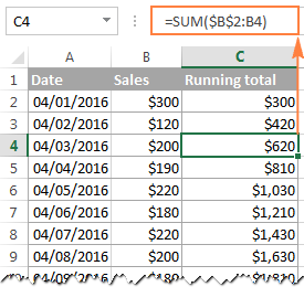
For example, to calculate the cumulative sum for numbers in column B beginning in cell B2, enter the following formula in C2 and then copy it down to other cells:
=SUM($B$2:B2)
In your running total formula, the first reference should always be an absolute reference with the $ sign ($B$2). Because an absolute reference never changes no matter where the formula moves, it will always refer back to B2. The second reference without the $ sign (B2) is relative and it adjusts based on the relative position of the cell where the formula is copied. For more information about Excel cell references, please see Why use dollar sign ($) in Excel formulas.
So, when our Sum formula is copied to B3, it becomes SUM($B$2:B3), and returns the total of values in cells B2 to B3. In cell B4, the formula turns into SUM($B$2:B4), and totals numbers in cells B2 to B4, and so on:
In a similar manner, you can use the Excel SUM function to find the cumulative sum for your bank balance. For this, enter deposits as positive numbers, and withdrawals as negative numbers in some column (column C in this example). And then, to show the running total, enter the following formula in column D:
=SUM($C$2:C2)
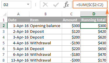
Strictly speaking, the above screenshot shows not exactly a cumulative sum, which implies summation, but some sort of "running total and running difference" Anyway, who cares about the right word if you've got the desired result, right? :)
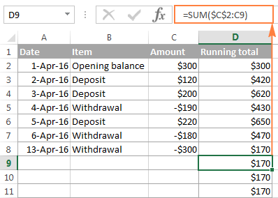
At first sight, our Excel Cumulative Sum formula looks perfect, but it does have one significant drawback. When you copy the formula down a column, you will notice that the cumulative totals in the rows below the last cell with a value in column C all show the same number:
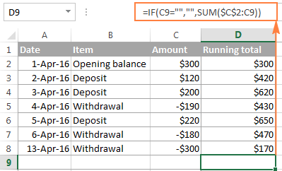
To fix this, we can improve our running total formula a bit further by embedding it in the IF function:
=IF(C2="","",SUM($C$2:C2))
The formula instructs Excel to do the following: if cell C2 is blank, then return an empty string (blank cell), otherwise apply the cumulative total formula.
Now, you can copy the formula to as many cells as you want, and the formula cells will look empty until you enter a number in the corresponding row in column C. As soon as you do this, the calculated cumulative sum will appear next to each amount:
How to make a cumulative graph in Excel
As soon as you've calculated the running total using the Sum formula, making a cumulative chart in Excel is a matter of minutes.
- Select your data, including the Cumulative Sum column, and create a 2-D clustered column chart by clicking the corresponding button on the Insert tab, in the Charts group:
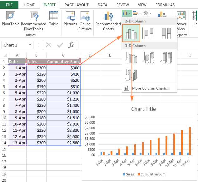
- In the newly created chart, click the Cumulative Sum data series (orange bars in this example), and right click to select Change Series Chart Type... from the context menu.
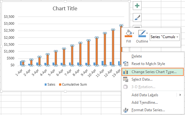
- If you are using a recent version of Excel 2013 or Excel 2016, select the Combo chart type, and click on the first icon (Clustered Column - Line) at the top of Change Chart Type dialog:
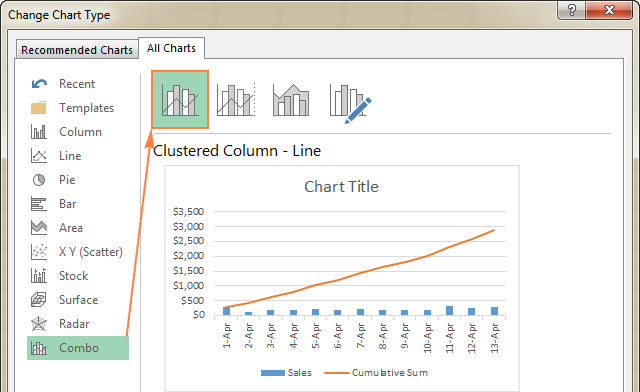
Or, you can highlight the Custom Combination icon, and choose the line type you want for the Cumulative Sum data series (Line with Markers in this example):
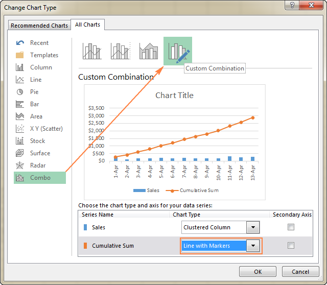
In Excel 2010 and earlier, simply select the desired line type for the Cumulative Sum series, which you've selected on the previous step:
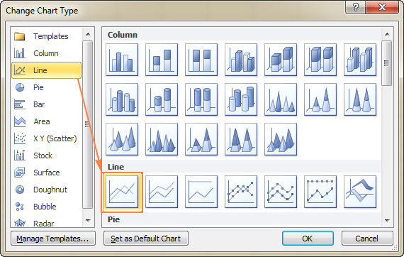
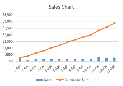
- Click OK, and evaluate your Excel cumulative chart:
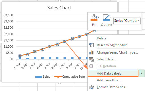
- Optionally, you can right-click the Cumulative Sum line in the chart, and select Add Data Labels from the context menu:
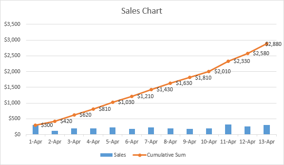
As the result, your Excel cumulative graph will look similar to this:
To embellish your Excel cumulative chart further, you can customize the chart and axes titles, modify the chart legend, choose other chart style and colors, etc. For the detailed instructions, please see our Excel charts tutorial.
This is how you do a running total in Excel. If you are curious to learn a few more useful formulas, check out the below examples. I thank you for reading and hope to see you again soon!
 by
by
96 comments
Editing a spreadsheet that has a cumulative sum column
I have a spreadsheet into which I have entered a series of transactions, and alongside each transaction amount I have a formula which gives the running total.
Lets say, at some point in the future, I notice that the order of the transactions is incorrect and I need to move one of them up to its correct position. So I insert a blank row at the appropriate point and I can then copy the transaction that is in the wrong place into this blank row, and then delete the original row. This works fine.
However, I had expected to be able to MOVE the transaction into the blank row by dragging, rather than COPY it and delete the original. When I MOVE the transaction, the relative reference does not update.
For example if row 4 has a cumulative total formula of =SUM($B$2:B4), and row 7 has a cumulative total formula of =SUM($B$2:B7), and I want to move the current row 7 transaction into the position currently occupied by the row 4 transaction, if I use "copy and delete", the formula copied from what was row 7 has its formula correctly changed to =SUM($B$2:B4) to reflect its new position.
If, instead I MOVE the row, then I end up with the formula =SUM($B$2:B8) in row 4. The relative reference has not been updated. (The reason it is now 8 not 7 is because it was updated when I added the new row at 4.)
Obviously it is no great hardship having to use "copy and delete", but I have to do this row rearrangement quite often, and I find myself using the MOVE method by mistake and then wondering why my spreadsheet is wrong.
Does anyone have any suggestions?
Hi! Maybe this article will be helpful: How to copy formula in Excel with or without changing references.
I am struggeling with sub totals with a sheet,could someone please guide me?
A have a number of columns, C is the equipment value, D is for damage, E fees and F Gross claim. We will pay all claims from a fund worth R1,500,000 after which the insurers will pay the balance, but all claims above a R250,000 cap will also be paid by the insurers.
The Fund depleting sum is "=SUM(IF(H8,MAX(IF(AND(H8>0,I8>0),J7-I8,J7-H8),0),0))", but the cap, the column priod to the fund's formula is "=MAX(IF(J14>$I$6,IF(AND(H15>0,H15$I$6,$I$6,H15)),$I$6-H15),0)". This particular formula carry on line by line down the sheet showing 250,000 which means my totas "Insurers Pay" formula and We pay do not realy add up properly.
Can I send the sheet as an example?
Without seeing your data, it is impossible to understand your formulas. In addition, the formulas contain references to columns that are not specified in your question. Please clarify your specific problem or provide additional details to highlight exactly what you need.
Great information here.
This is probably a simple one for the illuminati:
Suppose column C tracks profit gain and column D tracks profit losses. What would be the formula for column E tracking the ongoing balance?
It seems like it should be =SUM($C$2:C2)-SUM($D$2:D2) but I've apparently missed something.
Hi! If you copy this formula down the column, you will get the running profit total. To get just the profit total, change the cell references in the SUM formula. For example,
=SUM($C$2:C20)-SUM($D$2:D20)
How do I calculate the average of the total month at day 1, day 2, day 3 etc?
Hi!
If I understand your task correctly, you can use the AVERAGEIFS function and specify the desired days as the criteria.
Hi,
Thanks for the post.
I am trying to track if an event occurs more than 4 times per month (31 days?). Once the count is more than 3, I will use conditional formatting to color the cell. I have tried manipulating some SUMIF formulas, but I am very stuck.
Thus, I want to have a running total or occurrences, only if they occurred within a 31day bracket, continually.
A B C
Dates Did the event occur? "1" for yes, blank for no. Running Total of how many times the event occurred, in the past 31days.
2/10/2022 1 1
2/10/2022 1 2
15/10/2022 1 3
15/10/2022 1 4
16/10/2022 1 5
5/11/2022 1 4 (this is because now, the occurrences on 2/10 are more than 31 days ago)
7/11/2022 1 5
10/11/2022 5
10/11/2022 1 6
10/11/2022 1 7
10/11/2022 1 8
16/11/2022 1 7
11/12/2022 1
22/12/2022 0
24/12/2022 0
28/12/2022 1 1
29/12/2022
29/12/2022
29/12/2022
Any help is appreciated. Thanks.
Thanks for the post.
I am trying to track if an event occurs more than 4 times per month (31 days?)
Thus, I want to have a running total or occurrences, only if they occurred within a 31day bracket, continually.
A .......................B.....................................................................................C
Dates................Did the event occur? "1" for yes, blank for no..............Running Total of how many times the event occurred, in the past 31days
2/10/2022.........1.....................................................................................1
2/10/2022.........1.....................................................................................2
15/10/2022.......1.....................................................................................3
15/10/2022.......1.....................................................................................4
16/10/2022.......1.....................................................................................5
5/11/2022.........1.....................................................................................4.(this is because now, the occurrences on 2/10 are more than 31 days ago)
7/11/2022.........1.....................................................................................5
10/11/2022..............................................................................................5
10/11/2022......1......................................................................................6
10/11/2022......1......................................................................................7
10/11/2022......1......................................................................................8
16/11/2022......1......................................................................................7
11/12/2022..............................................................................................1 (this is because there has been no occurrence since 11/11)
22/12/2022..............................................................................................1
24/12/2022..............................................................................................1
28/12/2022.......1.....................................................................................2
29/12/2022
29/12/2022
29/12/2022
Any help is appreciated. Thanks.
Sorry, realized I had manually added the occurrences wrong - shows why I want to automate it.
Thanks for the post.
I am trying to track if an event occurs more than 4 times per month (31 days?)
Thus, I want to have a running total or occurrences, only if they occurred within a 31day bracket, continually.
A .......................B.....................................................................................C
Dates................Did the event occur? "1" for yes, blank for no..............Running Total of how many times the event occurred, in the past 31days
2/10/2022.........1.....................................................................................1
2/10/2022.........1.....................................................................................2
15/10/2022.......1.....................................................................................3
15/10/2022.......1.....................................................................................4
16/10/2022.......1.....................................................................................5
5/11/2022.........1.....................................................................................4.(this is because now, the occurrences on 2/10 are more than 31 days ago)
7/11/2022.........1.....................................................................................5
10/11/2022..............................................................................................5
10/11/2022......1......................................................................................6
10/11/2022......1......................................................................................7
10/11/2022......1......................................................................................8
16/11/2022......1......................................................................................7
11/12/2022..............................................................................................4 (this is because there has been only 4 occurrence since 11/11)
22/12/2022..............................................................................................1
24/12/2022..............................................................................................1
28/12/2022.......1.....................................................................................1
29/12/2022
29/12/2022
29/12/2022
Any help is appreciated. Thanks.
Hello!
To calculate a running total by condition, try this formula.
=SUM(($B$1:B2=1)* (IFERROR(DATEDIF($A$1:A2,A2,"D")>=0,0))* (IFERROR(DATEDIF($A$1:A2,A2,"D")<=31,0)))
You can learn more about calculating date diference in this article: Excel DATEDIF function to get difference between two dates.
Hi I'm trying to get a running accm. total for revenue over various sheets on an excel file. For each week I get the revenue and the following week I get another total and I want to keep adding them together as I pull new sheets. How would I do that?
for example;
sheet one -- total revenue
sheet two -- total revenue +total revenue of sheet one
sheet three -- total revenue + (sheet two total revenue + sheet one total revenue)
sheet four -- total revenue + (sheet three total revenue + sheet two total revenue + sheet one total revenue)
Hi!
Here is the article that may be helpful to you: 3-D reference in Excel: reference the same cell or range in multiple worksheets.
I want to set up a spreadsheet so that it totals values per week, i.e. on 12/2/22, I can see the sum of the values from 11/26/22-12/2/22. Then next week, I want it to total the sum of the values from 12/3/22-12/9/22 and so on and so forther.
Hi!
Write in cell B1 the formula SUM(A1:A7). Then select the range B1:B7 and drag the fill handle down the column. See for more information: How to copy formula in Excel.
Hi
Is there any function that will do running total values of same date and repeat again when new date starts
Hi!
You can calculate the amount for a certain date using the SUMIF function. When calculating the running total, use it instead of the SUM function.
I hope it’ll be helpful.
A B C D E
1 10 10
2 22 32
3 0 22
4 32 32
5 16 48
6 0 16
7 0 0
COUNTIF(B1:B7;">0")
RESULT = 3 from Column B
Require formula where
Result = 1
Which is determined as follows:
In Column C - Helper column
IF(B1+B2;"=0";0;B1+B3)
RESULT is 1
Formula required to get
RESULT =1
Without the Helper Column C
Thank you.
Hi!
I don’t know how you can get result 1. But the formula should be written like this
IF(B1+B2=0;0;B1+B3)
Read about using IF function in this tutorial.
Thanks for the walk through cheers
How would you calculate the cumulative totals if the dates in column A were not in order? Thanks!
have you ever found an answer for this
how to calculate Successive increase of $2 per 24h or part thereof for every next 24h with formula.
for example 1st 24 hours charges are $26 for next 24 hours charges will be $28 and so on.
Hi!
The information you provided is not enough to understand your case and give you any advice. How do you time your task?
Perhaps,
=24+(INT(A1/24)-1)*2
Hi in office 365 I'm updating my formulas to dynamic formulas, to avoid having to drag along each row/column and to avoid the risk of individual cells being affected by accidental changes (instead of locking the cells).
Now my challenge is the next:
I want to have a cumulative dynamic range without having to drag in the traditional way as described in this topic. I would assume this would be possible with a formula like =SUM(A$1:(A1:A10)) where the part after the first : would be the dynamic range --> ideally even in the form of =SUM(A$1:A#). But this does not result in a dynamic output, but only in SUM(A1:A10) c.q. SUM(A1:A#)
Thus I tried =SUM(A$1:INDIRECT(CELL("address",A#))) However the Cell function is not returning a dynamic range unfortunately.
My last brainfart was to try to have the output dependent on the position like =IF(A#0,SUM(A$1:A#),)
This does result in a dynamic output, however each position has the same value (SUM(A1:A#)) and is not a cumulative series.
Does anyone know of a solution?
Thank you! My question:
I have a complex table. Therefore, I am not aiming at creating additional column with cumulative sum.
Can I then, ask Excel to plot a cumulative sum line chart? i.e. the dataseries entry will specify cummulative figures from a (yet to be cumulatively summed) column?
thanks.
Hi!
A graph in Excel is built according to the data that is written in certain cells.
When I follow your example exactly, it doesn't work for me!
When I have got the formulas in each of the cells, eg in C4 it is =SUM($B$2:B4) it only adds B2and B4, missing out B3.
For cell B5, the formula is =SUM($B$2:B5) but it only adds B2 and B5, missing out B3 and B4.
Am I doing something wrong?
Hello!
The formula =SUM($B$2:B5) sums cells B2 through B5. You can check this using a calculator.
You can learn more about SUM function in Excel in this article on our blog.
This time, I really don't know how to solve it.
Columns: DateTime [A] | Values [B] | Codes [E]
So we have an ordered (DateTime) succession of values with several Codes IDs in the rows.
To try to make my life easier, I did my attempts in two different columns accordingly to plus [N] and minus [O] signs.
in [N] I need to sum the positive Values of that specific Code until it compares a value of the opposite sign in [B]. When the sign gets back to positive in [B], I need to SUM starting from zero. The same for the Negative column [O].
So far, with this in [N]
=IF($B2>0;SUMIFS($B$2:$B2;$E$2:$E2;$E2;$B$2:$B2;">0");"")
and this in [O]
=IF($B2<0;SUMIFS($B$2:$B2;$E$2:$E2;$E2;$B$2:$B2;"<0");"")
I was able to get something, but it doesn't start over.
But my real goal, is to actually be able to know after how many time periods (i.e. every 15 minutes) the Values for that specific Code go from its last same sign value
i.e.
6/06/2020 14:45; +255; apple
6/07/2020 14:45; -502; apple
6/08/2020 14:45; +841; apple
6/09/2020 16:45; -612; apple
I should find 192 (2days or 48h) for the positive side, and 200 (2days+2h)
Have a great day