The tutorial shows how to use the SUMIFS function in Google Spreadsheets to sum cells with multiple criteria. You will find a handful of real-life SUMIFS formula examples with AND as wells as OR criteria.
Google Spreadsheets provide two functions to conditionally sum cells, SUMIF and SUMIFS. Regular visitors of our blog are already familiar with SUMIF that we covered last week, and today we are going to have a closer look at its plural version.
The difference between SUMIF and SUMIFS is as follows:
SUMIF can add up cells based on just one condition. If it is what you want, please check out this tutorial: SUMIF in Google Sheets.
SUMIFS can sum cells based on two or more conditions. Further on in this tutorial, you fill find a simple explanation of SUMIFS syntax and formula examples for different data types.
Google Sheets SUMIFS function - syntax & basic uses
The SUMIFS function is Google Sheets is designed to sum numbers with multiple conditions. Its arguments are as follows:
Where:
- Sum_range(required) - the range to be summed.
- Criteria_range1 (required) - the range of cells to be evaluated by criterion1.
- Criterion1 (required) - the condition to be met by cells in criteria_range1.
- Criteria_range2, criterion2, … (optional) - additional ranges and criteria to test.
SUMIFS in Google Sheets - 3 things to remember
Using SUMIFS formulas in Google spreadsheets is quite easy. To prevent most common errors, just remember these three simple facts:
- The SUMIFS function adds up only those cells that meet all conditions, i.e. all of the specified criteria are true for a cell. This is commonly referred to as AND logic.
- Sum range and all criteria ranges should be equally sized, i.e. have the same number of rows and columns, otherwise your SUMIFS formula will throw a #VALUE error.
- Depending on the nature of your conditions, build your criteria appropriately:
- Text, wildcard characters and dates should be enclosed in quotation marks like "apples" or "*" or "4/19/2024".
- Numbers and cell references are not enclosed in quotation marks when used on their own.
- Logical operators with numbers, dates or text must be enclosed in double quotes like ">200", ">4/19/2024" or "<>apples" .
- Logical operators used together with cell references and other functions require the quotes to begin a text string and ampersand to concatenate and finish the string off. For example: ">"&B1 or ">="&TODAY().
Okay, that's enough theory, let's build some useful formulas already!
How to sum with multiple criteria (AND logic)
When it comes to summing cells with multiple criteria, you may find a lot of different suggestions in Google groups and other user communities.
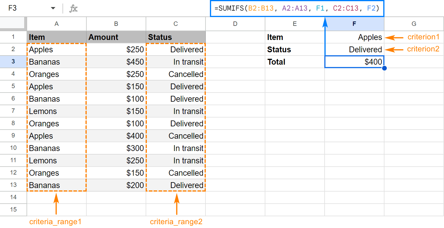
Let's say, you have a list of items in column A, amounts in column B, and delivery status in column C. Your goal is to get a total for a specific item with a certain delivery status, for example "apples" that are "delivered". How would you approach the task?
You may be surprised to know that many people still use array formulas for this purpose. For example, this one:
=ARRAYFORMULA(SUMPRODUCT((A2:A13="apples")*(C2:C13="delivered")*(B2:B13)))
What's wrong with this formula, you may ask me. Nothing except that it's excessively complex, difficult to understand and debug. It's like using a sledgehammer to crack a nut. Google Sheets SUMIFS function provides an easier way!
So, let's go ahead and define our arguments:
- Column A should contain "apples". Assuming we have data in rows 2 to 13, our criteria_range1 is A2:A13, and criterion1 is "apples".
- Column C should contain "delivered". Meaning, our criteria_range2 is C2:C13, and criterion2 is "delivered".
- Numbers to sum are in column B, so our sum_range is B2:B13.
Putting the arguments together, we get this simple formula:
=SUMIFS(B2:B13, A2:A13, "apples", C2:C13, "delivered")
To add more flexibility, you can input both criteria in separate cells, say F1 and F2, and refer to those cells:
=SUMIFS(B2:B13, A2:A13, F1, C2:C13, F2)
As shown in the screenshot below, our SUMIFS formula works perfectly!
Taking the example further, let's see how to use SUMIFS with other criteria types.
SUMIFS with logical operators
When your conditions are numbers or dates, use the comparison operators to express the criteria:
- equal to (= or omitted)
- not equal to (<>)
- greater than (>)
- less than (<)
- greater than or equal to (>=)
- less than or equal to (<=)
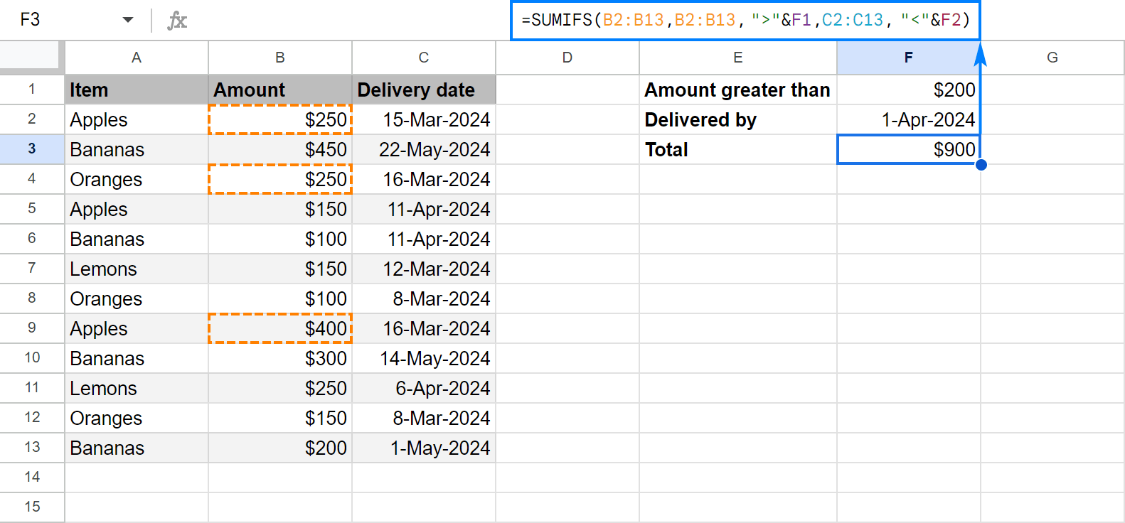
For example, to add up amounts in B2:B13 that are greater than or equal to 200 and delivered before 1-Apr-2024, use this formula:
=SUMIFS(B2:B13,B2:B13,">=200", C2:C13, "<4/1/2024")
In case you want to replace actual values with references to cells holding your criteria, please remember to enclose the logical operator in quotation marks and to concatenate the cell reference by using an ampersand:
=SUMIFS(B2:B13, B2:B13, ">="&F1, C2:C13, "<"&F2)
The screenshot below shows the result:
SUMIFS with other functions
In some situations, the conditions may depend on the results returned by some other functions. In this case, embed those functions in the criterion arguments of your SUMIFS formula.
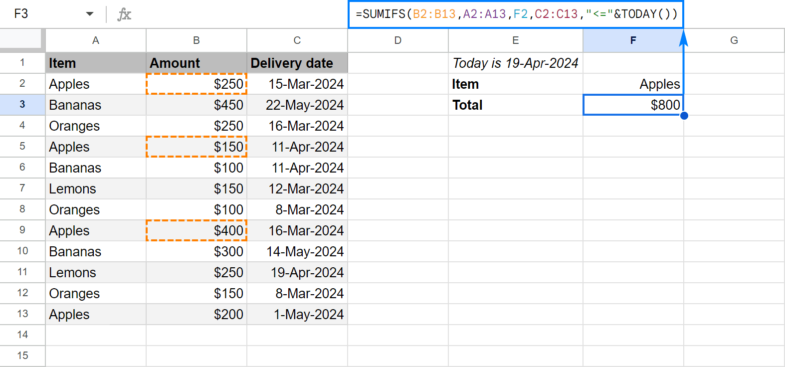
As an example, let's sum "apples" that are "delivered". In other words, the delivery date is up to and including today, so we concatenate the "less than or equal to" operator (<=) with the TODAY() function:
=SUMIFS(B2:B13,A2:A13,F2,C2:C13,"<="&TODAY())
And get the following result:
SUMIFS with blank and non-blank cells
To sum numbers in one column depending on whether a cell in another column is empty or not empty, use one of the following criteria:
- "=" to sum cells that are completely blank, i.e. contain absolutely nothing.
- "" to sum empty cells including zero length strings.
- "<>" to sum non-blank cells including zero length strings.
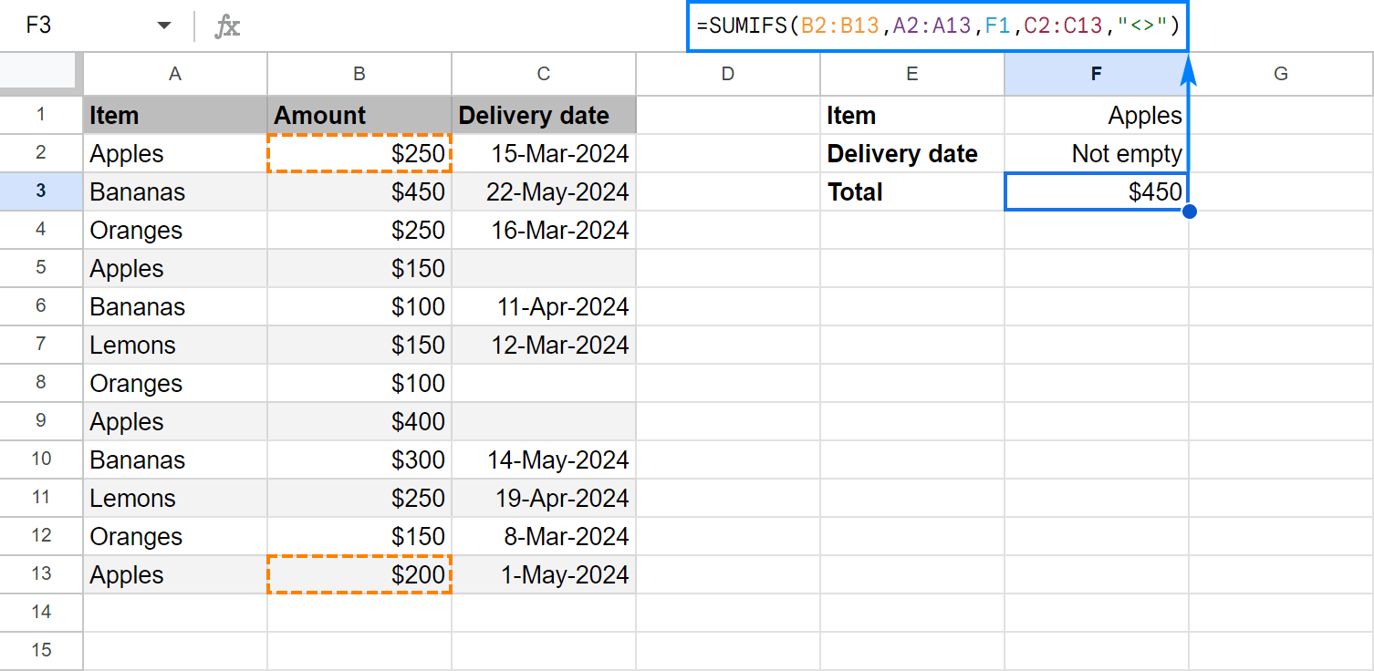
In case the Delivery date column contains some gaps, you may want to sum only those "apples" for which the delivery date is set, i.e. a cell in column C is not empty. The task can be accomplished with this formula:
=SUMIFS(B2:B13,A2:A13,"apples",C2:C13,"<>")
How to sum with multiple criteria (OR logic)
As you already know, by default, Google Sheets SUMIFS function works with AND logic - all conditions must match to be summed. In some situations, however, you may need to conditionally sum cells with OR logic, when any of the specified criteria is true. Below you will find a few possible ways to do this.
SUMIF with OR criterion (multiple criteria in the same column)
To sum cells with only a couple of criteria in the same column, you can simply add two SUMIF functions together.
For example, to sum the amounts in column B if column A is either "apples" or "bananas", use the SUMIF() + SUMIF() combination in its simplest form:
=SUMIF(A:A,"apples",B:B) + SUMIF(A:A,"bananas",B:B)
If you have three or more criteria, you may be looking for a more compact formula. For this, include the items in an array constant (aka inline array), use ArrayFormula to get a subtotal for each item, and wrap the whole construction into SUM() to add the subtotals together. For example:
=SUM(ARRAYFORMULA(SUMIF(A2:A13, {"apples", "bananas", "lemons"}, B2:B13)))
Instead of "hard-coding" the items in an array constant, you can enter them in individual cells, and include cell references in the array (in case of non-contiguous cells) or supply a range (in case of contiguous cells).
To better show you that our SUMIF formula works in exact accordance with the specified OR criteria, I've narrowed down the list to two items:
=SUM(ARRAYFORMULA(SUMIF(A2:A13, {E1, E2}, B2:B13)))
Or
=SUM(ARRAYFORMULA(SUMIF(A2:A13, E1:E2, B2:B13)))
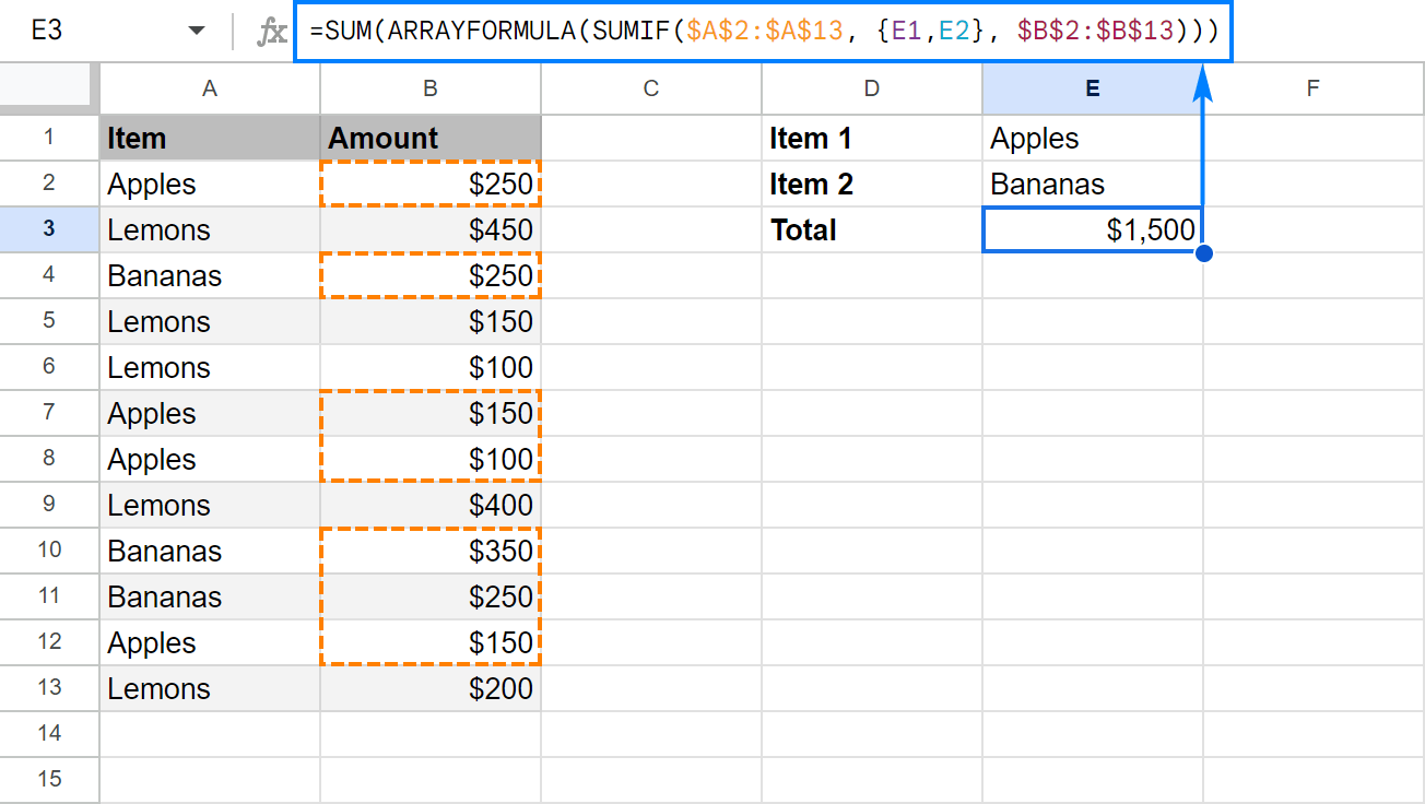
Instead of ArrayFormula, you can add up subtotals with the SUMPRODUCT function. For a short list of items, you can put it this way:
=SUMPRODUCT((A2:A13="apples") + (A2:A13="bananas"), B2:B13)
For multiple OR criteria (three or more items), you'd better use this syntax:
=SUMPRODUCT((A2:A13={"apples", "bananas"}) * B2:B13)
Replace the array elements with cells references, and you will get the most compact formula to sum cells with multiple OR criteria ever!
=SUMPRODUCT((A2:A13={E1, E2}) * B2:B13)
The screenshot below shows the result:
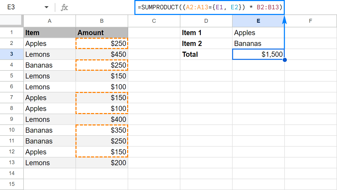
Four different formulas, the same result. Which one to use is the matter of your personal preference :)
SUMIF with OR criterion and results in different cells
If you'd like to have a subtotal for each item in a separate cell, take an array SUMIF formula discussed above, adjust the references, and cut off the SUM() part:
=ARRAYFORMULA(SUMIF(A2:A13, {"apples", "bananas", "lemons"}, B2:B13))
This will give you a sum for each item in a separate cell as shown in the screenshot below:
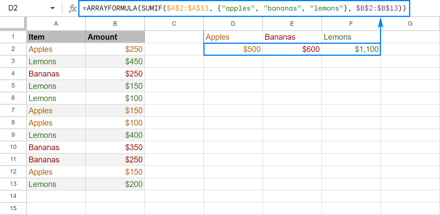
For the sake of clarity, you enter the formula only in the leftmost cell (D2 in this example), and Google Sheets will put the results into as many cells as many items there are in your array constant. Just make sure you have enough empty cells to the right, otherwise, the result won't be expanded and the formula will turn into an error.
If you'd rather have subtotals in a column, then separate the array elements with semicolons to make a vertical array:
=ARRAYFORMULA(SUMIF(A2:A13, {"apples"; "bananas"; "lemons"}, B2:B13))
And the results will be output vertically in a column:
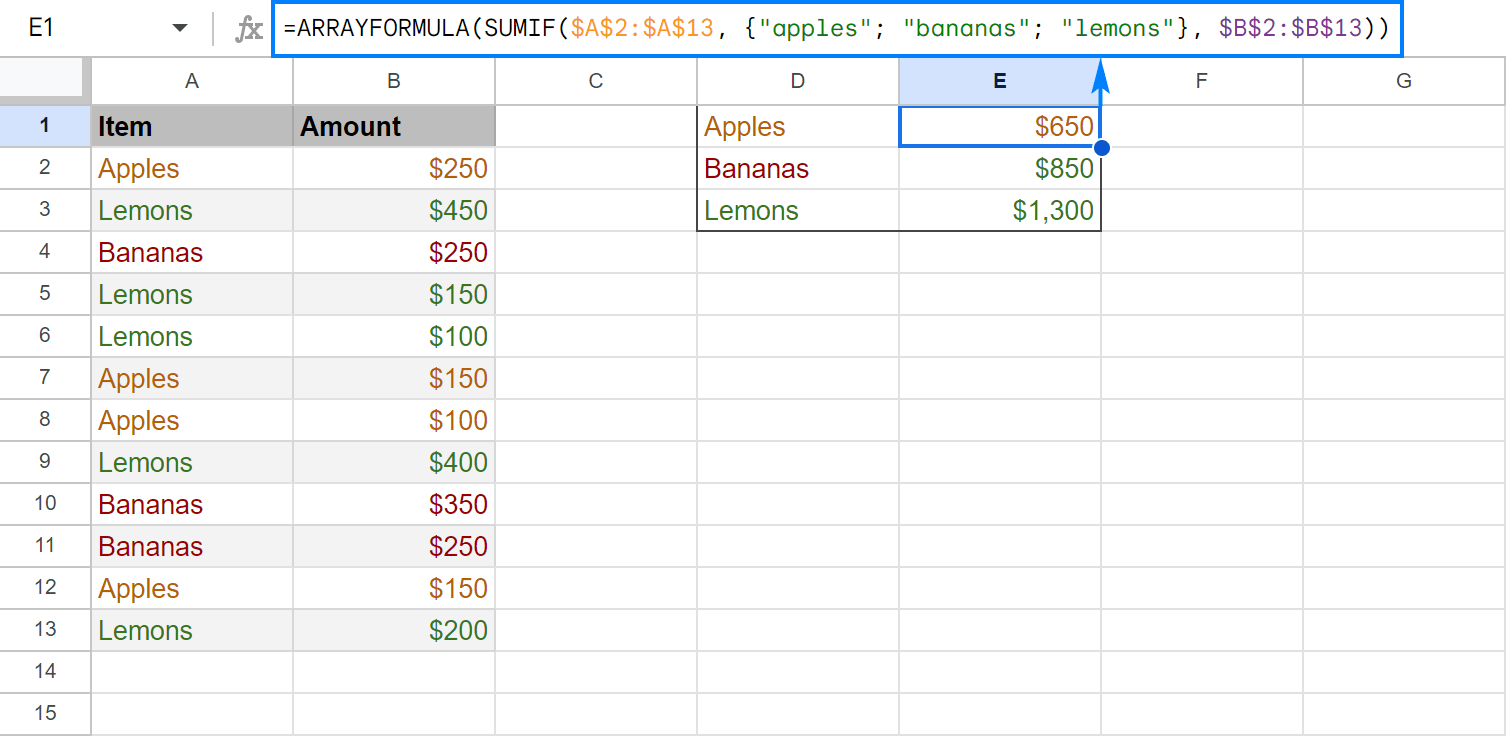
Tip. As usual, you can make your formula more flexible by replacing a hard-coded array with a range reference. That way, your users could type any items in the predefined cells, and you won't have to worry about updating your formula. For example, the formula shown in the screenshot above, can take the following shape:
=ARRAYFORMULA(SUMIF(A2:A13, D1:D3, B2:B13))
SUMIFS with OR criteria (multiple criteria in different columns)
This example shows how to sum numbers with several sets of conditions determined by the following logic.
- Within each set, all conditions must be true (AND logic)
- A cell is summed if any set of conditions is true (OR logic)
To make things easier to understand, please consider the following example. In our sample data set, supposing you want to sum amounts in column B if column A contains either "apples" OR "oranges" AND the delivery date in column C is "16-Mar-2018".
The most obvious way is to make two SUMIFS formulas to sum "apples" and "oranges" separately, and then add up the results:
=SUMIFS(B2:B13, A2:A13, "apples", C2:C13, "16-Mar-2024") +

SUMIFS(B2:B13, A2:A13, "oranges", C2:C13, "16-Mar-2024")
Or, you can enter your criteria in some cells, as shown in the screenshot below:
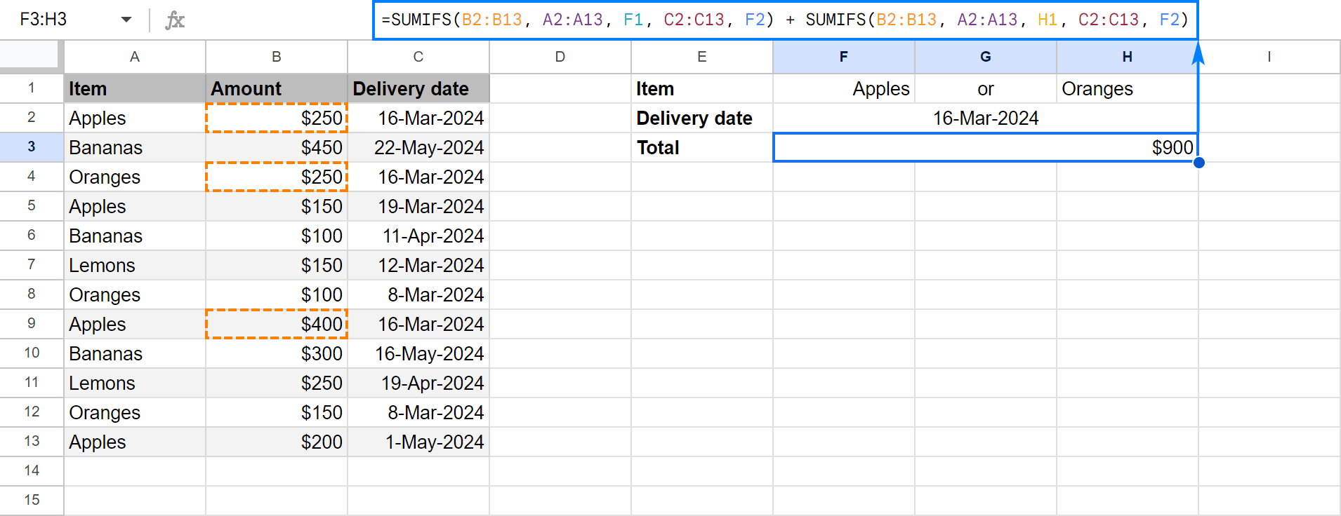
Regrettably, Google Sheets do not allow expressing multiple OR conditions using array constants, therefore we cannot make a plural version of our SUMIF with OR criteria formula. Luckily, there is another way to achieve the same result with a bit shorter formula - the SUPRODUCT function.
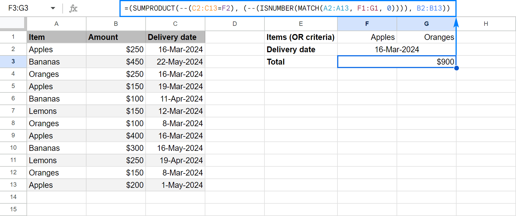
As an example, let's enter the desired delivery date (AND criterion) in F2 and items (OR criteria) in contiguous cells, say F1 and G1. Now, you can use the following formula to sum numbers in B2:B13 based on the above criteria:
Working from the inside out, here's what you do:=(SUMPRODUCT(--(C2:C13=F2), (--(ISNUMBER(MATCH(A2:A13, F1:G1, 0)))), B2:B13))
How this formula works
ISNUMBER(MATCH(A2:A13, F1:G1,0))
As the result, you'll get an array or TRUE and FALSE values (TRUE if any of the specified criteria is met, FALSE if none of the criteria is met).
Instead of a cell reference, you can enter the date directly in a formula by using DATEVALUE or DATE function. For example, C2:C13=DATEVALUE("3/16/2024") or C2:C13=DATE(2024,3,16)
In this formula, however, you cannot compare a range with a date directly, like C2:C13="3/16/2024" or C2:C13="16-Mar-2024", because you'd be comparing a cell with a date to a text string. Google Sheets won't understand that and you will most likely get a zero result.
If done correctly, this comparison will give you another array or TRUE and FALSE.
SUMPRODUCT will first multiply the elements of 3 arrays (two arrays of 0's and 1's and an array of numbers in B2:B13), and then sum the products. Because multiplying by 0 always yields 0, only the cells that have 1 in the first two arrays will "survive". As the result, only the amounts with the specified delivery date and item names will be summed.
This is how you use SUMIFS in Google Sheets to sum cells with multiple conditions. To have a closer look at the formulas discussed in this tutorial, I invite you to open our SUMIFS Google Sheets Examples. I thank you for reading and hope to see you on our blog next week!
Spreadsheet with formula examples
SUMIFS Google Sheets Examples (make yourself a copy)
 by
by
177 comments
Hello,
I am trying to build a formula but I'm not quite sure how to do it.
I want to automatically add up my expenses based on whether or not a checkbox is checked, but I also want to filter the criteria to a specific month.
My current (working) formula is =sumif(ARRAYFORMULA(TEXT(A3:A,"MMM-YYYY")),N7,G3:G) which gets me all of the numbers for the whole month (expenses and income) but I have 2 columns of checkboxes (Column I for income and Column J for expenses) that I want to add another criteria of if the expenses checkbox column is checked being the only cells that are being summed. But I also want them to be summed up based on the date range input from the formula above. I want to place these formulas in different boxes based on the date so I can compare one months expenses to another months expenses.
Is this possible?
Thank you.
Hello Ben,
For me to be able to assist you, please share a small sample spreadsheet with us (support@apps4gs.com) with 2 sheets: (1) a copy of your source data (2) the result you expect to get. The result sheet is of great importance as it gives us a better understanding than any text description.
I kindly ask you to shorten the tables to 10-20 rows.
Note. We keep that Google account for file sharing only and don't monitor its Inbox. Do not email there. Once you share the file, just confirm by replying to this comment.
I'll look into your task and try to help.
Buenos días,quisiera pedirte ayuda con la fórmula sumar.si.conjunto, la quiero usar en un inventario.
Producto. Cantidad. Movimiento. Producto. Cantidad inicial. Cantidad actual. Fecha v
Harina 2000. Salida. Harina. 10000. Form sumar si cjto( debería sumar o restar dependiendo si es entrada o salida).
Lo ví en un tutorial pero es antiguo y cambio la forma de escribir y me da error, error analisis , value. No sé cómo corregir. Agradezco tu ayuda.
Hello Gladys,
Sorry, we provide help in English only. If you're having difficulties with your SUMIFS formula, please reply with the exact formula you're using and specify the text of the error you see when hovering your mouse over the formula. I'll try to help.
Hello, please help:
COLUMN1 COLUMN2
Adult Dog 1
Adult Cat 2
Baby Dog 3
Baby Cat 4
Senior Dog 5
Senior Cat 6
How would I use SUMIFS to calculate, for example total Adults, or total Babies, BUT using a condition to sum the numbers in COLUMN2 by EXCLUDING those rows which have a certain string? Example, count all dogs except Senior, or count all animals except Baby Cat? Thanks you!
Hello Slava,
I can see 4 different tasks in your comment. For example, to sum all adults, the following formula will do: =SUMIFS(B2:B7, A2:A7, "*Adult*")
The same for babies.
To count all but seniors, you could use this one: =SUM(B2:B7)-SUMIFS(B2:B7, A2:A7, "*Senior*")
The same for all but baby cats.
Hello,
I am trying to build a workout summary for my workouts.
I have the raw data going into a tab "workouts" - This has "submission date" for the date of the workout entry.
Column B is type of workout (pushups, pullups, etc)
Column C is "reps"
Column D is "weight"
Column E is "time"
Reps, weight and time repeat to represent up to 10 "sets" of exercise. (Final column is AF)
I am trying to build a second tab, "workout summary", representing 1 week in each row, starting with 1/1/2024 as A2 for example, then 1/8/2024 in A3...
I want this to be a summary of total reps of each exercise done each week.
So if column A is "Week", Column B is "Pullups", Column C is "Pushups", etc.
I am trying to build a formula to sum the total number of pullups I did during the week, based on the data entered in "workouts"
Thanks in advance!
Hello Heath,
Sorry for the late reply, we were on holidays. If you still need help with your task, for me to be able to assist you, please share a small sample spreadsheet with us (support@apps4gs.com) with 2 sheets: (1) a copy of your source data (2) the result you expect to get. I kindly ask you to shorten the tables to 10-20 rows.
The result sheet is of great importance as it gives us a better understanding than any text description.
Note. We keep that Google account for file sharing only and don't monitor its Inbox. Do not email there. Once you share the file, just confirm by replying to this comment.
I'll look into your task and try to help.
I am a teacher and attempting to track data on Math Tests and Test Retakes using a Google Spreadsheet. I have set up a sheet that does basically everything I want, but I am having trouble with some "if this, then this, and then this" type statements to get my final data.
Column A = Student #
Column B = Score on original test
Column C = Score on the test retake
Column D = Score change from original test to retake test
Since my school is grading using Standards Based Grading, the students receive a 1, 2, 3, or 4 on a test. This means all of the scores in Column B will be either a 1, 2, 3, 4. I then total all of the students who receiveda 4 on the original test, 3 on the original test, etc. For instance, there are 30 students and 16 of them scored a 4 on the original test, 10 of them scored a 3, and 4 of them scored a 2. The "Received a 4" total will be 16 (there were 16 students that received a score of 4 on the test), Received a 3 total will be 10, and the Received a 2 total will be 4.
If a student scores a 1 or a 2 on the orignal test, he/she is forced to retake the test after reteaching and allowed the opportunity to increase his/her score. If a student scores a 3 on the original test, he or she can still retake the test in order to improve his/her score. I track all of the retake scores in Column C on my spreadsheet and total all of the scores of 4 on the retake, 3s, 2s, and 1s using the same method as listed above.
Where I struggle in my formulas is trying to do something like this ---- if the score in Column B is greater than the score in Column C, then use the score in Column B to total up the number of 4s, 3s, 2s, and 1s in Column B. BUT, if the score in Column C for a particular student is greater than the score in Column B for that student, I want to use the score in Column C in the total for Column B. For instance, let's take two students, #1 and #2. Student #1 scores a 4 on the original test and student #2 scores a 2 on the original test. The "Received a 4" total will be 1 and the "Received a 2" total will be 1. Student #2 retakes the test and scores a 3. I want my formula to look at the score in Column B and Column C and take the larger of those scores to use in the computation for the totals. In this instance, after the retake, I would have the following results: "Received a 4" = 1 and "Received a 3" = 1. The score of "received a 2" would no longer be present as the system did not total up the score for student #2 from Column B because Column B was lower than Column C. Since Column C had a higher score, the formula used the total from Column C to compute the overall totals.
I hope I am relaying what I desire correctly because I see it clearly in my mind. My guess is, there is a formula that can do this and I hope you all can help me. Thank you for your time and your effort on this task of mine as it has me stumped.
Hello Trigg,
Thank you so much for the detailed description of the task! Looks like a formula like this will help you out:
=COUNTIF(ARRAYFORMULA(IF(B2:B30 >= C2:C30, B2:B30, C2:C30)), 4)
It's for those who got 4 as a final result. Just make the copies and replace 4 with 3, 2 and 1 to get the count of students for other scores.
Is it possible to apply a function to the criterion range in SUMIFS?
Something like:
=SUMIFS(Transactions!$C:$C, month(Transactions!$B:$B), 11)
which doesn't work (gives: Array arguments to SUMIFS are of different size.)
Hi Tim,
It is MONTH that doesn't work with the range in this case.
Hi Tim,
I was solving a similar task and managed to make MONTH work by wrapping it in ARRAYFORMULA. Sorry I didn't think of this solution earlier.
Hi,
I am trying to return a sum by using SUMIFS, I have a requirement to use multiple criterion (S6:S17) so I used it with SUMPRODUCT but the result is zero. The formula is working fine with single criterion. Kindly advice
=SUMPRODUCT(SUMIFS(L:L,D:D,T6,A:A,S6:S17))
Hi Ali,
Try to modify your formula as shown in this part of the article.
Hello. Is there a way to use SUMIFS to add together numbers from multiple columns but based on criteria from other multiple columns? Even more complicated, can it be done in a header formula (like an array formula) that will work for an entire column?
Here's a very basic stripped down version of what I'm trying to do as an editable test sheet that is hopefully self-explanatory...
https://docs.google.com/spreadsheets/d/158wOjuhqNTOtR9TvE3I3t7356WQ7IHe2srtF2e50luc/
Thank you!!
Hello CC,
Sorry, your comment's got lost among all others. Do you still need help with the task?
i need to sum the number of quantity with the 2 criteria; check in and out and product name. the output should be number of check in of particular product. You missed to include an additional criterion in sum ifs with or & and.
Hi! Without seeing your data, it's hard to offer you a formula. I think the examples in the article above will help you.
Hi, I am trying to return a value based on two criteria. I have 3 columns of data. One column has the date, another column a numeric value and another column a letter denoting a code. I would like to display on another sheet the numeric value when the month in the column and the column with the code match it will return that value.
column 1 column2 column3
6-30-23 $1
7-31-23 $7 d
so if column 1 = month 7 and column 3 =d return the value of $7 to another sheet
I am not sure how to accomplish this. I would greatly appreciate any help, thanks so much!
Hi Tony,
It looks like you need to use the IF function for the task, with the AND logic specifically.
To add month as a criteria, use the MONTH function within IF.
Hello Natalia:
Can you help shed light on the correct function for (I think Sumif) for this problem:
ColB ColC ColD ColE ColF ColG ColS ColT
Fruits Qty Fruits Qty Fruits Qty Unique Fruits Qty Unique Fruits
Row12 Apples 15 Plums 3 Figs 18 Apples ??
Row13 Oranges 8 Coconuts 3 Grapes 9 Apricot ??
Row14 Dates 7 Peaches 8 Apples 9 Bananas ??
Row15 Figs 12 Cherries 24 Apricot 12 Cherries ??
Row16 Apricot 9 Bananas 9 Oranges 8 Coconuts ??
Row17 Peaches 14 Kiwi 12 Bananas 9 Dates ??
Row18 Apples 5 Peaches 6 Figs ??
Row19 Cherries 7 Grapes ??
Row20 Kiwi 8 Kiwi ??
Row21 Oranges ??
Row22 Peaches ??
Row23 Plums ??
For Column S I used function to sort the unique fruits: =sort(unique(filter(FLATTEN(B12:B20,D12:D20,F12:F20),FLATTEN(B12:B20,D12:D20,F12:F20)"")))
How do I sum for Column T?
Thanks in advance for your help.
Hello Eric,
Please share an editable sample spreadsheet with this data with us directly: support@apps4gs.com
Please include your SORT formula and the result you'd like to get. I'll look into your task and try to help.
Note. We keep that Google account for file sharing only and don't monitor its Inbox. Please do not email there. Once you share the file, just confirm by replying to this comment.
I am trying to do a SUMIFS formula. Situation is this.
I need the sum of several different cells (dollar amounts) to fall between the dates 1/1/2022 and 1/31/2022. Dates are speified in the column right before it (D:D for $$ and C:C for dates) I have this right now =SUMIFS(D:D, C:C ">=01/01/2022", ">=01/31/2022")
Please help
Hello Jacalin,
You missed a comma and one argument. Please pay attention to this part of the article to build the formula correctly.
HI,
I am using this formula with two regular conditions and then an array for an OR condition for that list. Here is the formula
=(SUMPRODUCT(--(DB_Date=$A$7)*(--(DB_Rev_Type=$F$1)), (--(ISNUMBER(MATCH(DB_Customer, filter(DB_Customer,DB_Date=$F$4,DB_Rev_Type=$F$1,DB_ARR=0), 0)))), DB_ARR))
What I am missing is the ability for cell F1 to be changed to "*" and the formula include all values in this condition (DB_Rev_Type=$F$1)
Thanks
Hi Matt,
Please try this formula:
=ARRAYFORMULA(SUMPRODUCT(--(DB_Date=$A$7),--(IF($F$1="*",IF(DB_Rev_Type<>"",TRUE,FALSE),DB_Rev_Type=$F$1)),--(ISNUMBER(MATCH(DB_Customer,FILTER(DB_Customer,DB_Date=$F$4,DB_Rev_Type=$F$1,DB_ARR=0),0))),DB_ARR))
I'm trying to do a sumifs with conditions, i have been trying for 2 weeks now, moving around parts, but i can't make it works!
I would love to have a bit of help, i can send my spreadsheet. Thank you.
=if(isblank(C5),"",
if(SUMIFS(Dividends_Liste!$M:$M,Dividends_Liste!$B:$B,$R$2,Dividends_Liste!$C:$C,$F$4,Dividends_Liste!$E:$E,C5,Dividends_Liste!$G:$G,$B$2,Dividends_Liste!$H:$H,$C$2)>"0",
if(search("Janv",D5),SUMIFS(Dividends_Liste!$M:$M,Dividends_Liste!$B:$B,$R$2,Dividends_Liste!$C:$C,$F$4,Dividends_Liste!$E:$E,C5,Dividends_Liste!$G:$G,$B$2,Dividends_Liste!$H:$H,$C$2)),
SUMIFS(Dividends_Liste!$M:$M,Dividends_Liste!$B:$B,$R$2,Dividends_Liste!$C:$C,$F$4,Dividends_Liste!$E:$E,C5,Dividends_Liste!$G:$G,$B$2,Dividends_Liste!$H:$H,$C$2)))
Or even something like that: =if(isblank(C5),"",
iferror(IF(regexmatch(D5,"May"),SUMIFS(Dividends_Liste!$M:$M,Dividends_Liste!$B:$B,$R$2,Dividends_Liste!$C:$C,$J$4,Dividends_Liste!$E:$E,C5,Dividends_Liste!$G:$G,$B$2,Dividends_Liste!$H:$H,$C$2),
if(SUMIFS(Dividends_Liste!$M:$M,Dividends_Liste!$B:$B,$R$2,Dividends_Liste!$C:$C,$J$4,Dividends_Liste!$E:$E,C5,Dividends_Liste!$G:$G,$B$2,Dividends_Liste!$H:$H,$C$2)>0,
SUMIFS(Dividends_Liste!$M:$M,Dividends_Liste!$B:$B,$R$2,Dividends_Liste!$C:$C,$J$4,Dividends_Liste!$E:$E,C5,Dividends_Liste!$G:$G,$B$2,Dividends_Liste!$H:$H,$C$2),"0"),"nul")))
What i want to do is: if month present in "D", i want the result of formula "sumifs" or "0" if no data yet, but if the formula "sumifs" is >0, without having the month in "D", i still want the result of the "sumifs" formula showing.
And if no month and formula "sumifs"=0, then i want "nul" as a result
Hello Angel,
Yes, please share an editable copy of your spreadsheet with us (support@apps4gs.com) with 2 sheets: (1) a copy of your source data, (2) the result you expect to get. The result sheet is of great importance as it gives us a better understanding than any text description. If you have confidential information there, you can replace it with some irrelevant data, just keep the format.
Note. We keep that Google account for file sharing only and don't monitor its Inbox. Please do not email there. Once you share the file, just confirm by replying to this comment.
I'll look into it and try to help.
Thank you for your fast reply, i sent a sharing link to your email. You have 3 sheets inside and the same formulas that i wrote here.
I hope it's understandable.
I want the main formula "sumifs" to be excecuted even if there is the month written or not. But if the month is in the future written, i want the result to be "nul" like that i can format and have "prediction" colors.
I even try with the today's date, but in one of my sheet it's 01/01/1900 for months so today will always be older than any days (even if i use month only and not full date)
I hope it's not too confusing...
Thank you very much
Thank you for sharing the file, Angel, I've got it.
I'll look into it and try to find a solution asap.
Angel,
I can see that your expected results are the same as the actual formula results. If you still need assistance, please adjust the numbers in your expected results accordingly.
I filled up all the chart, and the formula doesn't give the result i want. (only 0 everywhere)
The formula totally works but it's not what i want.
I tried to explain in a better way what i want underneath the table, let me know if you can find a solution or not.
Thank you very much for your time.
Thank you for specifying it, Angel.
I duplicated the sheet and put the formulas to Jan-Apr (F5:I7). F5 is different from your expected result because there's no Jan in D5, so I guess you just filled it incorrectly in the example. Please fill cells for other months accordingly.
Hope this helps :)
How can I include a cell reference date range in this formula.
=SUMIF($AU$2:$AU,A21,$AO$2:$AO)+SUMIF($AU$2:$AU,A24,$AO$2:$AO)
Hello Steve,
Sorry, what do you mean by a cell reference date range? Can you give an example and explain the task in more detail?
Hi Natalia,
We have a sheet with multiple tabs. We want one cell in one tab (Tab 1) to capture the number from cells in a column (example, column D) from another tab (Tab 2) only if certain conditions are met in other columns in Tab 2.
For example, cell A5 in Tab 1 will add all the numbers in column D of Tab 2 if column A of Tab 2 contains "apple" and column B of Tab 2 contains "Bread" and column C of Tab 2 contains "Flower". In addition, the information in columns A, B and C of Tab 1 are dropdown menus.
Is it possible with SUMIFS?
Hi Diego,
Based on the description, I believe it's possible. Only the formula will work with the values selected in those drop-downs (hidden values won't be considered).
I've been looking all over for some content like this!
I have a small grouping of data, but I need a cell that will sum only the top 42 highest numbers from Columns B, D, F and J, but of those, only the numbers that are >59.
I know the formula must be simple, I just can't find a good source to learn what I need.
Hello Alaric,
For me to be able to help you better, please create a sample spreadsheet with 2 sheets: (1) a sample of your data (2) the result you expect to get; and share it with us – support@apps4gs.com. I kindly ask you to shorten the tables to 10-20 rows. If you have confidential information there, you can replace it with some irrelevant data, just keep the format.
Note. We keep that Google account for file sharing only and don't monitor its Inbox. Please do not email there. Once you share the file, just confirm by replying to this comment.
I'll look into your task and do my best to help.
In the meantime, you can try applying this formula to your data in Google Sheets.
Thank you in advance for your help on this question. I have been elected the secretary of a very small not for profit organization and I am in charge of recording receivables and payables.
I am looking to expand my sumif formula (probably convert to a sumifs) to evaluate not only the value in column A (expense/income category), but also the date (particular year) in another column in another tab (same sheet). This way I am only returning summations from this year, or from a previous year depending on the value in a cell used for comparison (cell a1 contains the year 2021).
The formula I have now
=SUMIF(INDIRECT("Ledger!$B$2:$B"),$A6,INDIRECT("Ledger!$i$2:$I"))
It looks at my ledge column B contains my expense category, A6 is what I am comparing it against (if donation=donation return $100 etc.), If the evaluation is true, the formula returns the sum (only where true) of the amounts found in column I (on the ledger tab).
What I want to do now
my formula(s) exist on an actual vs, proposed budget page. I want to save this tab off as a yearly report (copy the tab). In addition to my current criterion I want to add one (or two) evaluations. I want to continue comparing the value in column A and add an additional comparison or comparisons on the date found in column A of my ledger tab. The evaluation should only sum values that occur in the specific range. Specifically September through August (i.e. 09/01/2021-08/31/2022). This will permit me to archive off a copy of my current active tab for record purposes. and I can update the active tab year comparison cells without having to zero out my ledger. By year comparison cells I am referring to two newly created cells on the active sheet for the date evaluation. They can have the values 09/01/2021 and 06/30/2022 respective.
Thank you in advance for your help.
-Brian
Hello Brian,
If I understand your task correctly, the example from this section may be what you need. If you're ready to add your dates to 2 new cells, you can refer to those cells when adding the criteria just like in that example. You will need to add 2 conditions: >= for 09/01/2021 and <= for 08/31/2022.
If you're still not sure how to do that, please create a small sample table (10-20 rows) with some dummy data and include the result you expect to get. Then share this file with us: support@apps4gs.com
Note. We keep that Google account for file sharing only and don't monitor its Inbox. Please do not email there. Once you share the file, just confirm by replying to this comment.
I'll look into your sample and help you with a formula.
Hello dear,
1.please how can I find the number of subscribers per subject from a data set where the number of subscribers is grouped by dates?
2. why do the values in a pivot table go horizontal?
thank you.
Hello Ene,
Hi! I have a super easy one for you but for some reason I just can't get my array formula to work. I need a list of sum of column C for each combination of Comumn A & Comumn B that currently exists.
Example data:
Lindsay Mitchelle 19
Staci Elvers 9
Shelia Jacobs 19
Staci Elvers 17
Lindsay Mitchelle 18
Shelia Jacobs 20
Lindsay Stamon 7
What I need the results to be is:
Lindsay Mitchelle 37
Staci Elvers 26
Shelia Jacobs 39
Lindsay Stamon 7
Here's a sheet with some more example data:
https://docs.google.com/spreadsheets/d/1GNgV_s_o5gclVGqi02bEKAdZKBz7ZCp8fbJe9_nBkdI/edit?usp=sharing
Hi Kristi,
Please add the desired result directly to the file. You see, I don't know whether you need it on the same sheet or other certain cells. Also, do you use a list of all names that appear in a column somewhere? If so, please include it as well. Thank you.
Hi goodmorning. Can you help me in formula I'm a beginner on this field.
this is my formula
=SUMIFS('Order File'!E:E,"1299"'Order File'!F:F,"GOLD WATCH",'Order File'!D:D,"DELIVERED")
i need the total for the gold watch that was delivered and the amount is 1299, but there are other gold watch that has other amount. do i need to use "IF" function inside "SUMIFS? thank you
Hi Lloyd,
As far as I can see, you need to change your arguments places. Please look through this section to build the formula correctly.
Hey Guyz, can anyone help with this formula?
=SUMIFS(ImportRange("1j_7JWjcC9I5I_erUOCj0TnVKn7mvveBdPuy89pWKJb8",'Master Deal Data'!$C$2:$C), ImportRange("1j_7JWjcC9I5I_erUOCj0TnVKn7mvveBdPuy89pWKJb8",'Master Deal Data'!$BG$2:$BG),$B3, ImportRange("1j_7JWjcC9I5I_erUOCj0TnVKn7mvveBdPuy89pWKJb8",'Master Deal Data'!$BH2:$BH),2021)
Here $B3 is the month name like 'January'...
If I try CountIfs, it works perfectly but when I try this formula i.e. SUMIFS it shows me 'Argument must be a range'.
If i use this formula directly in the sheet with which I am linking using Importrange function, it works too...
Please anyone help.
Hi Ritessh,
SUMIFS doesn't work this way. Instead, use QUERY + IMPORTRANGE. QUERY knowns how to sum records as well.
How do I use SUMIF to only a select and take the sum of the two smallest/largest/middle values?
Hello!
To find the multiple largest values, use the LARGE function. For the smallest values, use the SMALL function. To find the largest or smallest average, you must first calculate the average and then use these functions. Also take a look at the guide How to find top or bottom N values in Excel.
Hi I would like to combine these 2 formulas into 1 using SUMIFS or whatever it is I need but I am having a hard time. They both work correctly individually.
The first formula below looks through a column of hours and sums them only if they fall within range of a month. For example, it will sum only if hours were entered in January 2022. (A1 is the date for example 1/1/2022)
=sumifs(G7:G805,H7:H805,">="&DATE(YEAR(A1),MONTH(A1),1),H7:H805,"<="&EOMONTH(A1,0))
The 2nd formula sorts through a column and sums them only if a "SUBJECT TAUGHT" matches. (In my example it sums up only if Pathology was lectured.
SumIF(I7:I37,"Pathology",G7:G37)
Basically I am trying to nest or combine them so that it sums up the subject taught only if it falls within a month/date range.
Hi Danny,
If I understand you correctly, you just need to add the criteria_range & the criterion from the second formula into the first one:
=sumifs(G7:G805,H7:H805,">="&DATE(YEAR(A1),MONTH(A1),1),H7:H805,"<="&EOMONTH(A1,0),I7:I805,"Pathology")
However SUMIFS requires all arguments to be of the equal size, so you'll have to extend I7:I37 to I7:I805.
If this doesn't work for you, please share a small sample spreadsheet with us (support@apps4gs.com) with 2 sheets: (1) a copy of your source data (2) the result you expect to get (the result sheet is of great importance and often gives a better understanding than any text description). I kindly ask you to shorten the tables to 10-20 rows.
Note. We keep that Google account for file sharing only and don't monitor its Inbox. Once you share the file, just confirm by replying to this comment.
I'll look into it.
Hi, I'm having a similar issue. I have two sheets within a document: Sheet 1, "Pedidos" with a list of transactions showing date, quantity and price in the columns; Sheet 2, "Sumario Mensal" with a summary of products sold within the month for all of 2022.
When I use SUMIFS to calculate quantity "quantidade" sold within a date range, it returns the correct value: =SUMIFS(Pedidos!$C$3:$C,Pedidos!$A$3:$A,">="&F$1,Pedidos!$A$3:$A,"="&F$1,Pedidos!$A$3:$A,"<="&EOMONTH(F$1,0),Pedidos!$B$3:$B,"="&B3)
However, when I try to combine both formulas Sheets doesn't recognize the second formula as criteria_range 3, criterion. It keeps reading it as criteria_range 2. Have you ever seen anything like this?
I'll share the Sheet with the email you mentioned and if you guys can help me, it would be awesome!
Hi Pauline,
I'm sorry but I don't see any spreadsheet from you. Please share it directly with support@apps4gs.com and let me know when you do so, I'll look into it.
Hi Natalia,
i would like to have a formula to SUM a range in column D with criteria in column F (with text "x" or any number), the SUM are from row D2:D6.
i was try with this formula LOOKUP(1;1/(F2:F10);F2:F10) to find the last filled cell but i can not found how to combine with the SUM formula just to SUM from D2:D6 with said criteria.
with the criteria i do expect to able to calculate or SUM until any criteria as filled cell in column F. (text or any number)
A B C D E F
1 BALANCE PROFIT PROP+BAL WD LAST BALANCE TO SUM
2 100,00 13,00 113,00 1,30 111,70
3 111,70 14,52 126,22 1,45 124,77
4 124,77 16,22 140,99 1,62 139,37
5 139,37 18,12 157,48 1,81 155,67
6 155,67 20,24 175,91 2,02 173,89 x
7 173,89 22,61 196,49 2,26 194,23
8 194,23 25,25 219,48 2,53 216,96
9 216,96 28,20 245,16 2,82 242,34
10 242,34 31,50 273,84 3,15 270,69
WD up to "x" : 8,21
i do appreciate i you can share me the formula and many thanks for your kind support.
salam,
agus.
Hi Agus,
Try this formula:
=SUM(INDIRECT("$D$2:"&CELL("address";INDEX($D$2:$D$10;MATCH(FALSE;($F$2:$F$10="");0)))))
Wow....
this is really amazing formula, first i put as a normal formula and the result is ERROR with error message #VALUE!.
i was try to execute every single formula on those but still error then i realize that this is an array formula so i press CTRL-SHIFT-ENTER when executing the formula and it is working fine.
really really appreciate for quick response and thanks a bunch for the shared formula.
salam,
agus.
Agus,
I'm really sorry, I did forget to mention that it's an array formula! Glad to know you figured it out though – hope it didn't take too long :)
Hi, I am at my wits end. I have been trying to use countifs and sumifs to generate results in a table with no luck. Long story short, My data sheet is A1:K150, Column G has a dollar value (Dollar Amount), Column G, text/number combo (reason code) and Column J is text (Action Taken)
Example 1 that I could get Reason code is R13, I needed to count the times Reason code R13 was taken as a loss
Formula used with success is =COUNTIFS($H$3:$H$150,"R13",$J$3:$J$150, "Loss")
Now what I am trying to do is take the sum of the amount in column g and include it to the same results. Rather than count how many, I would like to sum to total of Column G where Column H is matches the reason code and column J is the action taken. IE Sum of items for R13 taken as loss.
Any help would be greatly appreciated.
Hi Les,
You'll find the solution to your task in this part of the article.
Thank you, I totally missed that. I figured it out after reviewing.
My pleasure :)
So I did a Sumifs function to add up day pay within the date range of the pay period...easy stuff because it's a basic sum.
What I would love to do (but can't quite figure it out) if write something similar but to subtract (clock in and clock out times) also within a date range.
I'm just savy enough to be dangerous...am I wasting my time trying to figure this out? Is it even possible to find a difference in two cells with date range criteria?
Hello Brenda,
For me to be able to help you, please create a sample spreadsheet with 2 sheets: (1) a sample of your data (2) the result you expect to get; and share it with us – support@apps4gs.com. The result sheet is of great importance and often gives us a better understanding than any text description. I kindly ask you to shorten the tables to 10-20 rows. If you have confidential information there, you can replace it with some irrelevant data, just keep the format.
Note. We keep that Google account for file sharing only and don't monitor its Inbox. Please do not email there. Once you share the file, just confirm by replying to this comment.
I'll look into your task and do my best to help.
Hi! I have a very complex formula (for me) that works in excel, but not Sheets. Can anyone show how to convert this for Sheets? It appears that I need the OR logic for the value arrays in SUMIFS and COUNTIFS, but my childish attempts to solve this have failed.
The article gives two options for OR logic using the non-S version, but it seems I still need to retain the S version of these functions. Any help is appreciated.
=IFERROR(SUM(SUMIFS(Sets!H:H,Sets!E:E,A9,Sets!C:C,{235,364,405,412,416,423,469},Sets!J:J,">="&OSS!$B$3,Sets!G:G,">"&$B$4,Sets!F:F,">="&$B$5))/SUM(COUNTIFS(Sets!E:E,A9,Sets!C:C,{235,364,405,412,416,423,469},Sets!J:J,">="&OSS!$B$3,Sets!G:G,">"&$B$4,Sets!F:F,">="&$B$5)),"")
I solved my issue using the formula below. Regexmatch is needed for SUMIFS I guess. Along with some shuffling of the functions.
=IFERROR(ArrayFormula(SUMIFS(Sets!H:H,Sets!E:E,A9,REGEXMATCH(Sets!C:C,"^(235|364|405|412|416|423|469)$"),TRUE,Sets!J:J,">="&OSS!$B$3,Sets!G:G,">"&$B$4,Sets!F:F,">="&$B$5))
/SUM(ARRAYFORMULA(COUNTIFS(Sets!E:E,A9,Sets!C:C,{235,364,405,412,416,423,469},Sets!J:J,">="&OSS!$B$3,Sets!G:G,">"&$B$4,Sets!F:F,">="&$B$5))),"")
Hello, In the spreadsheet below, on the first sheet called "Payouts", I am currently using Sumif in column B to total up values in column H from the second sheet called "Worksheet" if the name in the drop down column A matches any of the names in "Worksheets" column A.
I want to add a criteria that the Checkbox in column D in "Worksheet" be checked (=True) to include that row in the sum.
https://docs.google.com/spreadsheets/d/1qowl-flGEafWZJCvlf07GCrOWqsfdo68w8XA_S8Uad0/edit?usp=sharing
Hello Alex,
Try this formula:
=SUMIFS(Worksheet!H$3:H$100,Worksheet!A$3:A$100,A2,Worksheet!D$3:D$100,TRUE)
Hello,
from AL to BO i have scores (they range from 1 to 3) and from BS to CV i have the matching values either a or b or c. I would like to match total scores for a, b, or c for each row (one individual who completes a test).
I have tried many formulas that at best gives me a 0 or an error.
for example:
=SUMIFS(BS3:CV3;"a";AL3:BO3) gives a 0
=SUMIFS(AL2:AO2,BS2:BT2,"a") gives an #ERROR
am I trying something impossible to solve or could you provide me with some hints?
Thanks in advance for your time.
Hello Giulia,
For me to be able to help you, please create a sample spreadsheet with 2 sheets: (1) a sample of your data (2) the result you expect to get; and share it with us – support@apps4gs.com. The result sheet is of great importance and often gives us a better understanding than any text description. I kindly ask you to shorten the tables to 10-20 rows. If you have confidential information there, you can replace it with some irrelevant data, just keep the format.
Note. We keep that Google account for file sharing only and don't monitor its Inbox. Please do not email there. Once you share the file, just confirm by replying to this comment.
I'll look into your task and do my best to help.
Hey, how can I make this work for even or odd rows? Here’s what I’ve come up so far, but it says the argument must be a range:
=SUMIF(ISEVEN(ROW(C62:C76)),""&"",ISEVEN(ROW(A62:A76)))
Hey Dyn,
To sum numbers from the even rows, try a formula like this:
=SUM(FILTER(C62:C76,ISEVEN(ROW(C62:C76))))
If this doesn't work as you expect, for me to be able to help you, please consider sharing an editable copy of your spreadsheet with us (support@apps4gs.com) with 2 sheets: (1) a copy of your data (2) the result you expect to get (the result sheet is of great importance and often gives us a better understanding than any text description). I kindly ask you to shorten the tables to 10-20 rows. If you have confidential information there, you can replace it with some irrelevant data, just keep the format.
Note. We keep that Google account for file sharing only and don't monitor its Inbox. Please do not email there. Once you share the file, just confirm by replying to this comment.
I'll look into your task.
This was extremely useful! Thank you so much!
The equations with provided examples was so much clearer than other "support" I had found previously.