Do you know how to sum numbers in a certain column when a value in another column meets any of the specified conditions? In this article, you will learn 3 different ways to do SUMIF using multiple criteria and OR logic.
Microsoft Excel has a special function to sum cells with multiple conditions - the SUMIFS function. This function is designed to work with AND logic - a cell is added only when all of the specified criteria are TRUE for that cell. In some situations, however, you may need to sum with multiple OR criteria, i.e. to add a cell when any of the conditions is TRUE. And this is when the SUMIF function comes in handy.
SUMIF + SUMIF to sum cells equal to this or that
When you are looking to sum numbers in one column when another column is equal to either A or B, the most obvious solution is to handle each condition individually, and then add the results together:
In the table below, suppose you want to add up sales for two different products, say Apples and Lemons. For this, you can supply the items of interest directly in the criteria arguments of 2 different SUMIF functions:
=SUMIF(A2:A10, "apples", B2:B10) + SUMIF(A2:A10, "lemons", B2:B10)
Or you can enter the criteria in separate cells, and refer to those cells:
=SUMIF(A2:A10, E1, B2:B10) + SUMIF(A2:A10, E2, B2:B10)
Where A2:A10 is the list of items (range), B2:B10 are the numbers to sum (sum_rage), E1 and E2 are the target items (criteria):
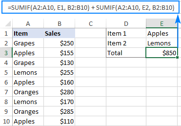
How this formula works:
The first SUMIF function adds up the Apples sales, the second SUMIF sums the Lemons sales. The addition operation adds the sub-totals together and outputs the total.
SUMIF with array constant - compact formula with multiple criteria
The SUMIF + SUMIF approach works fine for 2 conditions. If you need to sum with 3 or more criteria, the formula will become too big and difficult to read. To achieve the same result with a more compact formula, supply your criteria in an array constant:
Please remember that this formula works based on OR logic - a cell is summed when any single condition is met.
In our case, to sum sales for 3 different items, the formula is:
=SUM(SUMIF(A2:A10, {"Apples","Lemons","Oranges"}, B2:B10))
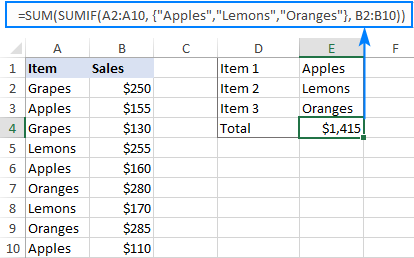
In the above screenshot, the conditions are hardcoded in an array, meaning you will have to update the formula with every change in the criteria. To avoid this, you can input the criteria in predefined cells and supply to a formula as a range reference (E1:E3 in this example).
=SUM(SUMIF(A2:A10, E1:E3, B2:B10))
In Excel 365 that supports dynamic arrays, it works as a regular formula completed with the Enter key. In pre-dynamic versions of Excel 2019, Excel 2016, Excel 2013 and earlier, it should be entered as an array formula with the Ctrl + Shift + Enter shortcut:
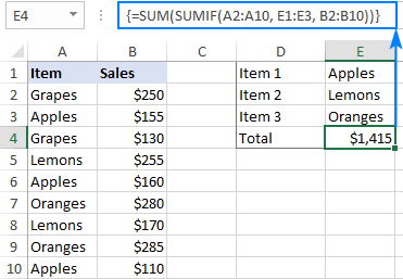
How this formula works:
An array constant plugged into SUMIF's criteria forces it to return multiple results in the form of an array. In our case, it's 3 different amounts: for Apples, Lemons and Oranges:
{425;425;565}
To get the total, we use the SUM function and wrap it around the SUMIF formula.
SUMPRODUCT and SUMIF to sum cells with multiple OR conditions
Don't like arrays and are looking for a normal formula that would allow you to sum with multiple criteria in different cells? No problem. Instead of SUM, use the SUMPRODUCT function that handles arrays natively:
SUMPRODUCT(SUMIF(range, crireria_range, sum_range))
Assuming the conditions are in cells E1, E2 and E3, the formula takes this shape:
=SUMPRODUCT(SUMIF(A2:A10, E1:E3, B2:B10))
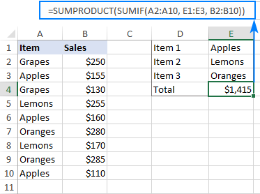
How this formula works:
Like in the previous example, the SUMIF function returns an array of numbers, representing the sums for each individual condition. SUMPRODUCT adds these numbers together and outputs a final total. Unlike the SUM function, SUMPRODUCT is designed to process arrays, so it works as a regular formula without you having to press Ctrl + Shift + Enter.
SUMIF using multiple criteria with wildcards
Since the Excel SUMIF function supports wildcards, you can include them in multiple criteria if needed.
For example, to sum sales for all sorts of Apples and Bananas, the formula is:
=SUM(SUMIF(A2:A10, {"*Apples","*Bananas"}, B2:B10))
If your conditions are supposed to be input in individual cells, you can type wildcards directly in those cells and provide a range reference as criteria for the SUMPRODUCT SUMIF formula:
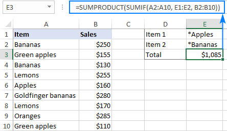
In this example, we put a wildcard character (*) before the item names to match any preceding sequence of characters such as Green apples and Goldfinger bananas. To get a total for items that contain specific text anywhere in a cell, place an asterisk on both sides, e.g. "*apple*".
That's how to use SUMIF in Excel with multiple conditions. I thank you for reading and hope to see you on our blog next week!
Practice workbook for download
SUMIF multiple criteria (.xlsx file)
 by
by
63 comments
How would i go about Simplifying =((E7*$B7)+(E8*$B8)+(E9*$B9)+(E10*$B10)+(E11*$B11)+(E12*$B12)+(E18*$B18)+(E19*$B19)+(E21*$B21)+(E23*$B23)+(E24*$B24)+(E25*$B25)+(E26*$B26)+(E27*$B27)+(E28*$B28)+(E29*$B29)+(E30*$B30)+(E31*$B31)+(E32*$B32)+(E33*$B33)+(E40*$B40)+(E43*$B43)+(E46*$B46)+(E60*$B60)+(E63*$B63)+(E65*$B65)+(E66*$B66)+(E68*$B68)+(E69*$B69)+(E70*$B70)+(E71*$B71)+(E75*$B75)+(E78*$B78)+(E79*$B79)+(E80*$B80)+(E90*$B90)+(E34*$B34)+(E35*$B35)+(E36*$B36)+(E37*$B37)+(E47*$B47)+(E48*$B48)+(E49*$B49)+(E50*$B50)+(E51*$B51)+(E53*$B53)+(E55*$B55)+(E61*$B61)+(E54*$B54)+(E57*$B57)+(E58*$B58))
I need to break it down into =If(a5="c",B5*E5,0) but need it to do this for the whole of column A and B to total into 1 cell
Hi! Based on your description, it is hard to completely understand your task. However, I’ll try to guess and offer you:
(E7*$B7)*(A7="c")+(E8*$B8)*(A8="c")+... etc.
Hi,
Thanks for all the info/help... just wondering if you can tell me which function to use in this case: I want to add amounts in column A if either column B, C, D, E contain "x". "X" is a destination from a table in column AA (AA1:AA10). What would be the most efficient way to do this?
Thanks!
Hello! If I understand your task correctly, try the following SUMPRODUCT formula with multiple criteria:
=SUMPRODUCT(--(((B2:B10="x")+(C2:C10="x")+(D2:D10="x")+(E2:E10="x"))>0),A2:A10)
I would like to sum under both an and AND an or condition. Is this possible?
For example If the text in column A is either x OR y, AND the text in column B is z, then Sum column C.
Hi! Use the SUMPRODUCT function for this combination of AND and OR conditions. The formula might look as follows:
=SUMPRODUCT(((A1:A10="x") + (A1:A10="y")) * (B1:B10="z") * C1:C10)
Look for the example formulas here: Excel SUMPRODUCT function with multiple criteria.
Thanks
Hi,
Sum with Sumifs isn't working when there are two criteria in two or more criteria range
Hi Alexander
I have two formulas that I'd like your assistance with please:
1. What formula should I use to allow the sum of multiple text options (potential, yes and no) in column AE. I tried the below but it doesn't work.
=SUMIFS('WCC Sites'!Z3:Z84, 'Sites'!AE3:AE84, {"Potential", "Yes", "No"}, 'Sites'!H3:H84, "=23/24")
2. How can I shorten the below? There's two worksheets (Sites & Stone), each with three options (potential, yes and no) that I would like the sum of the price for (Q2:Q86).
=SUMIF('WCC Sites'!AE2:AE85, "Potential", 'Sites'!Z2:Z85) + SUMIF('Sites'!AE2:AE85, "Yes", 'Sites'!Z2:Z85) + SUMIF('Sites'!AE2:AE85, "No", 'Sites'!Z2:Z85) + SUMIF('Stone'!V2:V86, "Potential", 'Stone'!Q2:Q86) + SUMIF('Stone'!V2:V86, "No", 'Stone'!Q2:Q86) + SUMIF('Stone'!V2:V86, "Yes", 'Stone'!Q2:Q86)
Many thanks
Hi! I can't check your formula, but it should return 3 values. Use the SUM function.
=SUM(SUMIFS('WCC Sites'!Z3:Z84, 'Sites'!AE3:AE84, {"Potential", "Yes", "No"}, 'Sites'!H3:H84, "=23/24"))
You can use this in the second formula as well. For example:
SUM(SUMIF('Sites'!AE2:AE85, {"Yes","No"}, 'Sites'!Z2:Z85))
does anybody now how to solve the following problem:
How to sum-up values considering two column with each multiple critera, e.g. sales revenue per (1) market per (2) segment,
for (1) want to include US and France, but not UK
for (2) want to include apples & peaches but no bananas
Thanks for help
Hi! You can find the examples and detailed instructions here: How to use Excel SUMIFS and SUMIF with multiple criteria.
Dear Sir,
can we sumifs formula so find the sum in data where there unique number in between. But this detials will not have the same length in the entire data
Hi! To ensure clear understanding of your task, can you provide an example of the source data and the desired result you are aiming for?
Hello,
I am requesting help for how to shorten the formula below but receive the same result.
I have a worksheet of data in "CT10 raw data" sheet relating to job numbers with cost, job type, job number, etc. I need to sum the cost for the job numbers that are not in a list of job numbers on worksheet "CT10". They are roughly 50 jobs numbers and i want to sum the ones that are not. in the list but the formula ends up being super long after listing out each crieria and criteria range. Is there a way to group the criteria together?
For Example:
Job Numbers:
22132
43214
87685
43296
Raw Data:
22132 $500
43214 $342
87685 $234
43296 $576
67345 $568
=SUMIFS('CT10 Raw Data'!$S$5:$S$2393,'CT10 Raw Data'!$B$5:$B$2393,""&'CT10'!$A$2,'CT10 Raw Data'!$B$5:$B$2393,""&'CT10'!$A$3,'CT10 Raw Data'!$B$5:$B$2393,""&'CT10'!$A$4,'CT10 Raw Data'!$B$5:$B$2393,""&'CT10'!$A$5,'CT10 Raw Data'!$B$5:$B$2393,""&'CT10'!$A$6,'CT10 Raw Data'!$B$5:$B$2393,""&'CT10'!$A$7,'CT10 Raw Data'!$B$5:$B$2393,""&'CT10'!$A$8,'CT10 Raw Data'!$B$5:$B$2393,""&'CT10'!$A$9,'CT10 Raw Data'!$B$5:$B$2393,""&'CT10'!$A$10,'CT10 Raw Data'!$B$5:$B$2393,""&'CT10'!$A$11,'CT10 Raw Data'!$B$5:$B$2393,""&'CT10'!$A$12,'CT10 Raw Data'!$B$5:$B$2393,""&'CT10'!$A$13,'CT10 Raw Data'!$B$5:$B$2393,""&'CT10'!$A$14,'CT10 Raw Data'!$B$5:$B$2393,""&'CT10'!$A$15,'CT10 Raw Data'!$B$5:$B$2393,""&'CT10'!$A$16,'CT10 Raw Data'!$B$5:$B$2393,""&'CT10'!$A$17,'CT10 Raw Data'!$B$5:$B$2393,""&'CT10'!$A$18,'CT10 Raw Data'!$B$5:$B$2393,""&'CT10'!$A$19,'CT10 Raw Data'!$B$5:$B$2393,""&'CT10'!$A$20,'CT10 Raw Data'!$B$5:$B$2393,""&'CT10'!$A$21,'CT10 Raw Data'!$B$5:$B$2393,""&'CT10'!$A$22,'CT10 Raw Data'!$B$5:$B$2393,""&'CT10'!$A$23,'CT10 Raw Data'!$B$5:$B$2393,""&'CT10'!$A$24,'CT10 Raw Data'!$B$5:$B$2393,""&'CT10'!$A$25,'CT10 Raw Data'!$B$5:$B$2393,""&'CT10'!$A$26,'CT10 Raw Data'!$B$5:$B$2393,""&'CT10'!$A$27,'CT10 Raw Data'!$B$5:$B$2393,""&'CT10'!$A$28,'CT10 Raw Data'!$B$5:$B$2393,""&'CT10'!$A$29,'CT10 Raw Data'!$B$5:$B$2393,""&'CT10'!$A$30,'CT10 Raw Data'!$B$5:$B$2393,""&'CT10'!$A$31,'CT10 Raw Data'!$B$5:$B$2393,""&'CT10'!$A$32,'CT10 Raw Data'!$B$5:$B$2393,""&'CT10'!$A$33,'CT10 Raw Data'!$B$5:$B$2393,""&'CT10'!$A$34,'CT10 Raw Data'!$B$5:$B$2393,""&'CT10'!$A$35,'CT10 Raw Data'!$B$5:$B$2393,""&'CT10'!$A$36,'CT10 Raw Data'!$B$5:$B$2393,""&'CT10'!$A$37,'CT10 Raw Data'!$B$5:$B$2393,""&'CT10'!$A$38,'CT10 Raw Data'!$B$5:$B$2393,""&'CT10'!$A$39,'CT10 Raw Data'!$B$5:$B$2393,""&'CT10'!$A$40,'CT10 Raw Data'!$B$5:$B$2393,""&'CT10'!$A$41,'CT10 Raw Data'!$B$5:$B$2393,""&'CT10'!$A$42,'CT10 Raw Data'!$B$5:$B$2393,""&'CT10'!$A$43,'CT10 Raw Data'!$B$5:$B$2393,""&'CT10'!$A$44,'CT10 Raw Data'!$B$5:$B$2393,""&'CT10'!$A$45,'CT10 Raw Data'!$B$5:$B$2393,""&'CT10'!$A$46,'CT10 Raw Data'!$B$5:$B$2393,""&'CT10'!$A$47,'CT10 Raw Data'!$B$5:$B$2393,""&'CT10'!$A$48,'CT10 Raw Data'!$B$5:$B$2393,""&'CT10'!$A$49,'CT10 Raw Data'!$B$5:$B$2393,""&'CT10'!$A$50,'CT10 Raw Data'!$B$5:$B$2393,""&'CT10'!$A$51,'CT10 Raw Data'!$B$5:$B$2393,""&'CT10'!$A$52)
Hello!
Use the SUMPRODUCT function to find the sum by condition. Use the MATCH function to check if the Job Numbers on the two sheets match.
Here is an example of a formula:
=SUMPRODUCT(--ISERROR(MATCH('CT10 Raw Data'!A1:A10,Data!A1:A10,0)),'CT10 Raw Data'!B1:B10)
I hope my advice will help you solve your task.
=(SUMIF('sheet1'!I2:I,"PT",'sheet1'!K2:K)*('sheet1'!L2:L))
I have to multiply numbers from column 1 with column 2 and them display the total sum
Hi!
You can calculate the sum of the products of the columns with the function SUMPRODUCT.
Good Day
Hope you can assist me,
When I use the following formula "=SUMIFS($Y:$Y,$B:$B, ">="&$X$1,$B:$B, "<="&$Y$1,$A:$A,$E2)" [$Y:$Y,$B:$B, - different workbook data] to calculate a value between two dates (X&Y) where the dates are in a fixed cell it only works when the data sheet that I'm getting the data from is open (Different Workbook). I had the same issue with this previously and was advised too use the "SUM(IF(" function instead of the "SUMIFS"
When I use the same Formula detail as with the SUMIFS function with the SUM(IF( it duplicates the values or returns an error
Is there a way i can use this SUMIFS or SUM(IF( correctly so that it does not return an error when the database workbook is closed
Hope this makes sense
Regards
Hi!
The Excel functions you are using can only get data from open workbooks. Your problem can be solved with VBA.
Dear
Like dsum work with two cell condition - can we used sumif two cell condition
excel formula to:
input data from cell B3 into cell D3, IF cell C3 does not equal criteria_1 OR does not equal criteria_2
Figured it out:
=SUMIFS(D3,B3,"criteris_1",D3,"criteria_2")
Hi!
The answer to your question can be found in this article: Excel IF OR statement with formula examples.
=SUM(SUMIFS(J2:J2646,F2:F2646,{"RUH-G1","RUH-G2"},G2:G2646,{"RUH-G1","RUH-G2"},H2:H2646,{"RTO"}))
Please help me not received right result.
Hi!
What data do you use and what result do you want to get?
Hi team, I am hoping you can help! It seems like a complex ask from me, but it might be super easy for someone who knows excel!
I have a large data set (800,000+ points). In my data set, I have;
Column 1 Column 2
Person 1 Treatment Cost 1
Person 2 Treatment Cost 1
Person 2 Treatment Cost 2
Person 2 Treatment Cost 3
Person 3 Treatment Cost 1
Person 3 Treatment Cost 2
Person 4 Treatment Cost 1
Person 5 Treatment Cost 1
Person 6 Treatment Cost 1
Person 6 Treatment Cost 2... etc etc
How would I sum the treatment cost for each person in the large data set using these functions?
Thank you!!!
MCM :)
Hi!
You need to find the sum with one condition. Therefore, you can use this guide: How to use SUMIF function in Excel with formula examples.
The formula might look like this:
=SUMIF(A1:A1000,"Person 1",B1:B1000)
I hope I answered your question.
Hi, How would you add data from two different criterias from two different ranges ?
Hi!
I am not sure I fully understand what you mean. Could you please describe it in more detail?
Hi-
I'm trying to add up how many different 'shot types' & 'complexities' I have and I can figure out how many times each shot type shows and complexity shows up but I can't figure out how to multiply it by the 'number of shots' I have for each category. ie: some cells have multiple shot counts.
=COUNTIFS(SEQUENCES!R:R,"Character",SEQUENCES!Q:Q,"VE")
shot type: character
complexity: VE
# Shots: 10
How do I add a multiplier? Do I need to use a different formula like SUMIFS or PRODUCT SUM?
Thanks,
J
Hi!
I am not sure I fully understand what you mean. I can assume that you need to find unique values without duplicates. Then I recommend this article: How to count unique values in Excel.
The formula provides me a return with a count of how many times each instance came up but I have a column I need to multiply that count by.
ie: Let's say there were 3 instances of shot type 'character' with a complexity of 'VE' but I have a shot count in those rows in a separate column of 5 shots each. The result that formula would give me would be 3 when I would actually need it multiplied by the number of shots which should then give me a total of 15.
So shot type is column R, complexity is column Q and I need to multiply that count by # of shots in another column. How do I add a multiplier?
Does that make sense?
Hi!
If I got you right, you need to use the SUMIFS formula:
=SUMIFS( [# Shots range] , SEQUENCES!R:R,"Character",SEQUENCES!Q:Q,"VE")
I hope it’ll be helpful.
Hi-
Thank you for that but I'm not understanding this part in the formula and excel won't accept it: [# Shots range]. I was thinking it would be more like this but it's not working either :
=SUMIFS(SEQUENCES!R:R,"Character",SEQUENCES!Q:Q,"VE"*SEQUENCES!S:S)
column S would contain different numeric values that I need to multiply the count of each instance by.
Thanks,
J
Hi!
I thought you would carefully read the article I recommended to you. The first parameter of the SUMIFS function is the column you are summing (number of shots). If this is not what you wanted, please describe the problem in more detail. If in your example the number of shots in 3 cells will be 4, 8 and 3 then what do you want to multiply, and what will be the result?
Thanks for your helpful articles. Very clear and well presented. I am trying to use the SUMIF formula to extract a total value from 1 column using a qualifying value detailed in another column between defined limits eg 1.60 to 2.0. I tried using "2.0" which gives an error message. I then tried SUMIFS but this appears to need values in 2 different columns to work. Is there a further article that would help here please? You can see the spreadsheet on this link if it helps. https://docs.google.com/spreadsheets/d/1BgZqQ-R5PGkoRtVwStJN-pl9TH57LIBDqpZPvA6WIoU/edit?usp=sharing The cell in question is D6 and E5 will need a similar solution ( I have used a simple work around for the time being but this will only work if I do not want to add further analysis). Thanks and regards Peter
Hello!
If I understand your task correctly, the following formula should work for you:
=SUMIFS($E$11:$E$1002,$D$11:$D$1002,">1.6",$D$11:$D$1002,"<2")
You can learn more about SUMIFS in Excel in this article on our blog.
"Count the number of unique IDs for which "received" is written." Exactly. Now you have undestood. Thank you.
The source data are below and the expected result is 1.
For the data below in two column, the formula result should be 1 eventhogh the ID5596326 appears 6 times and "received" 2 times.
5596326 attempted
5596326 delivered
5596326 received
5596326 received
5596326 sent
5596326 Wrong Number
Hello!
Your explanations are still not very clear. I'll try to guess. Count the number of unique IDs for which "received" is written.
=IFERROR(ROWS(UNIQUE(FILTER(A2:A100,B2:B100="received"))), 0)
You can read more about how to calculate unique values in this article.
I would like to request your assistance in developing an Excel formula.
I would like to count only the first occurrence in which an ID number appears in a column and also the text "received" appears in the same record (row) for that ID.
For example, if ID 5596326 occurs 6 times and "received" occurs 2 times for that ID.
For this ID, the answer would be 1.
What would be the formula?
This has really stumped me, and I would appreciate your help.
Hello!
If I understand your task correctly, the following formula should work for you:
=IF(COUNTIFS(A:A,A2,B:B,"received")>0,1,"")
I hope this will help, otherwise please do not hesitate to contact me anytime.
If the data, with a header row, consists of 100 records, with an ID column and a results column, how is the range or ranges specified?
Hi,
If I got you right, the formula below would help you with your task:
=IF(COUNTIFS($A$2:$A$101,A2,$B$2:$B$101,”received”)>0,1,””)
After that, you can copy this formula down along the column.
This formula =IF(COUNTIFS($A$2:$A$101,A2,$B$2:$B$101,”received”)>0,1,””) does not answer the question that I am asking. This formula results in a count of 1 on a single row for an ID in one colum and when "received" appears in an other column.
But my question is different. Take this example in which the ID is identical, but "received" appears twice. The same ID might appear 10 times and "received" 4 times. The problem is the same.
How for a single ID that may appear many times can a formula be written to produce one distinct result of 1 for an ID when the ID and "received" may appear more than once?
So the result that I am looking for is not 1 per row in which "received" appears, but 1 per distinct ID when the ID and "received" may appear multiple times as in the example.
5596326 attempted
5596326 delivered
5596326 received
5596326 received
5596326 sent
5596326 Wrong Number
The result that I am looking for can be achieved by filtering the workbook on "received," copying the filtered result to another worksheet, and remove duplicate rows by ID. Then I would just look at the resulting number of rows in teh worksheet and that would be the total number of distinct cases for a single ID and "received" having occurred at least once.
But I am looking for a formula to do that instead of going through the filtering and unduplicating procedure.
The result you need is
=IF(COUNTIFS($A$1:$A2,A2,$B$1:$B2,”received”)>0,"",IF(COUNTIFS($A$2:$A$101,A2,$B$2:$B$101,”received”)>0,1,""))
Hello!
Sorry, I do not fully understand the task. Write an example of the result you want to get. You sent a file with an example of source data, but there is no example of the expected result. Do you want to get a list of IDs? I cannot guess.
i am trying to set formulae for calculating figures in various sheets for dated 1st to 30th of month in which all the figures are in same column i,e for example A5 of sheet 1,sheet 2.
please suggest me the formulae
Hello!
I think our article on 3D links in Excel will help you.
Dear Sir,
RID NAME Jan 01 Jan 02 Jan 03 Jan 04 Jan 05 Jan 06 Jan 07 Jan 08 upto Dec 31
10001 Name 1 # # # # P A A A P P
10002 Name 2 # # # # P A A A P P
10003 Name 3 # # # # P A A A P P
10004 Name 4 # # # # P A A A P P
10005 Name 5 # # # # P A A A H H
10006 Name 6 # # # # P A A A P P
# HOLIDAY
H Half day
A absent
P present
RID MONTH No of Days Present
10001 JANUARY ?
How to get no of days present with given parameters.
Thanks - D. Phani Kumar
Hello!
I’m sorry but your task is not entirely clear to me. Could you please describe it in more detail? What result do you want to get? Thank you!
Dear Sir,
if some body asks how may days absent/present in a month or total year, to answer this, i will take his RID and MONTH / FROM TO DATES. SHEET holds current years attendance of employees both new and old.
RID 01/01/2020 02/01/2020 …. 31/12/2020 # HOLIDAY
1001 P P P H Half day
1002 # H A A absent
1003 P P P P present
Hello!
If I understand your task correctly, calculate the number of "P" for the desired period for the employee using the COUNTIFS function. Then multiply by the number of hours that corresponds to P. For other letters - the same.
Hi,
I have the following formula
=IF(ISNUMBER(SEARCH("fred",B12))*ISNUMBER(SEARCH("saturday",L12)),E12*$M$2*$R$5,"")
This give the desired output for fred and Saturday but I need to add the same again but for fred and Sunday, which would also change the refernce M2 to R2. So the equiv' formula for fred and Sunday is
=IF(ISNUMBER(SEARCH("fred",B12))*ISNUMBER(SEARCH("sunday",L12)),E12*$R$2*$R$5,"")
How do I combine the two?
Thanks
Ian
Hello!
Add a condition to test the value of cell L12
=IF(ISNUMBER(SEARCH(“saturday”,L12)), IF(ISNUMBER(SEARCH(“fred”,B12))*ISNUMBER(SEARCH(“saturday”,L12)),E12*$M$2*$R$5,””), IF(ISNUMBER(SEARCH(“fred”,B12))*ISNUMBER(SEARCH(“sunday”,L12)),E12*$R$2*$R$5,””))
I hope it’ll be helpful.
Thanks for good guidance
12D, 6N, R, N, L, D, SL, R, N, D, 9N. CAN YOU PLEASE HELP ME TO SUM THIS ALPHANUMERICS, BUT BY OMITTING THE LETTERS I SHOULD GET THE ANSWER AS = 27.
THANKS A LOT
Hello!
To extract and sum all single and double digit numbers from text, use the formula
=SUM(IF(ISNUMBER(--MID(A1,ROW($1:$93),2)),--MID(A1,ROW($1:$93),2),""))
Hope this is what you need.
Hi!
Thank you for the details and steps above!
I am having some issues with the Sum+sumif and sumproduct formulas, when I enter in the formula with the range E1:E3 I get a '0' value returned. I went back to the steps again and continuously checked the formula, but still get the '0' value.
What other areas/values should I check?
Thank you,
E
Hi!
It's difficult to say anything certain without seeing your data and formula. For starters, please check if the numbers you are summing are really numbers and not numbers stored as text. If you add them up with a simple formula like =A1+A2+A3..., does it work? If this simple calculation works fine, then the problem is definitely with the Sum+Sumif formula.
You can send your source data and expected result to us at support@ablebits.com, and we will try to figure it out.
Hello!
The information you provided is not enough to understand your case and give you any advice, sorry. For me to be able to help you better, please describe your task in more detail. Please specify what you were trying to find, what formula you used and what problem or error occurred. Give an example of the source data and the expected result.
It’ll help me understand it better and find a solution for you.