Trying to build an IF statement with wildcard text, but it fails every time? The problem is not in your formula but in the function itself - Excel IF does not support wildcard characters. However, there is a way to get it to work for partial text match, and this tutorial will teach you how.
Whenever you want to perform partial or fuzzy matching in Excel, the most obvious solution is to use wildcards. But what if a specific function that you need to use does not support wildcards characters? Sadly, Excel IF is one of such functions. This is especially disappointing considering that other "conditional" functions such as COUNTIF, SUMIF, and AVERAGEIFS work with wildcards perfectly well.
Luckily, it is not the obstacle that can stop a creative Excel user :) By combining IF with other functions, you can force it to evaluate a partial match and get a nice alternative to an Excel IF wildcard formula.
Why Excel IF function with wildcard not working
In the sample table below, supposing you want to check whether the IDs in the first column contain the letter "A". If found - display "Yes" in column B, if not - display "No".
It seems like including wildcard text in the logical test would be an easy solution:
=IF(A2="*a*","Yes", "No")
But regrettably it does not work. The formula returns "No" for all the cells, even those that contain "A":
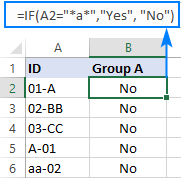
Why does a wildcard IF statement fail? From all appearances, Excel doesn't recognize wildcards used with an equal sign or other logical operators. Taking a closer look at the list of functions supporting wildcards, you will notice that their syntax assumes a wildcard text to appear directly in an argument like this:
=COUNTIF(A2:A10, "*a*")
Excel IF contains partial text
Now that you know the reason why a wildcard IF formula fails, let's try to figure out how to get it to work. For this, we'll simply embed a function that accepts wildcards in the logical test of IF, namely the COUNTIF function:
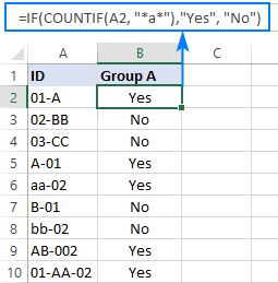
With this approach, IF has no problem with understanding wildcards and flawlessly identifies the cells that contain either "A" or "a" (since COUNTIF is not case-sensitive):
=IF(COUNTIF(A2, "*a*"),"Yes", "No")
This formula goes to B2, or any other cell in row 2, and then you can drag it down to as many cells as needed:
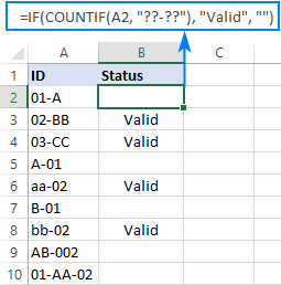
This solution can also be used to locate strings of a specific pattern. Assuming only the IDs consisting of 2 groups of 2 characters separated with a hyphen are valid, you can use the "??-??" wildcard string to identify them:
=IF(COUNTIF(A2, "??-??"), "Valid", "")
How this formula works:
For the logical test of IF, we use the COUNTIF function that counts the number of cells matching the specified wildcard string. Since the criteria range is a single cell (A2), the result is always 1 (match is found) or 0 (match is not found). Given that 1 equates to TRUE and 0 to FALSE, the formula returns "Valid" (value_if_true) when the count is 1 and an empty string (value_if_false) when the count is 0.
IF ISNUMBER SEARCH formula for partial matches
Another way to force Excel IF to work for partial text match is to include either the FIND or SEARCH function in the logical test. The difference is that FIND is case-sensitive while SEARCH is not.
So, depending on whether you want to treat lowercase and uppercase as the same or different characters, one of these formulas will work a treat:
Case-insensitive formula for partial match:
Case-sensitive formula for partial match:
As both functions are designed to perform a "cell contains" type of match, wildcards aren't really needed in this case.
For example, to detect IDs containing "A" or "a", the formula is:
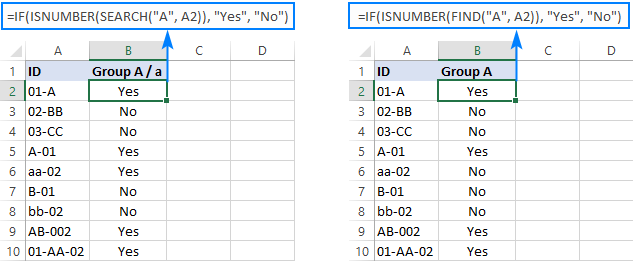
=IF(ISNUMBER(SEARCH("A", A2)), "Yes", "No")
To only search for a capital "A" and ignore "a", the formula is:
=IF(ISNUMBER(FIND("A", A2)), "Yes", "No")
In B6 in the screenshot below, you can observe the difference in the result:
How this formula works:
At the heart of the formula, there is a combination of ISNUMBER and SEARCH (or FIND):
ISNUMBER(SEARCH("A", A2))
The SEARCH function looks for the specified text ("A" in this example) and returns its position within a string in A2. If the text is not found, a #VALUE error is returned. As both SEARCH and FIND are designed to perform a "cell contains" type of match, wildcards aren't really needed in this case.
The ISNUMBER function converts a number to TRUE and any other value including error to FALSE. The logical value goes directly to the logical test of IF. In our case, A2 contains "A", so ISNUMBER returns TRUE:
IF(TRUE, "Yes", "No")
As the result, IF returns the value set for the value_if_true argument, which is "Yes".
Excel IF OR statement with wildcards
Need to identify cells that contain one of wildcard text strings? In this case, you can combine the classic IF OR statement with the COUNTIF or ISNUMBER SEARCH formula discussed above.
For example, to search for "aa" OR "bb" in A2 ignoring the letter case and return "Yes" if either is found, use one of these formulas:
=IF(OR(ISNUMBER(SEARCH("aa", A2)), ISNUMBER(SEARCH("bb", A2))), "Yes", "")
or
=IF(OR(COUNTIF(A2, "*aa*"), COUNTIF(A2, "*bb*")), "Yes", "")
Adding up two COUNTIF functions will also work. In this case, the plus sign works like the OR operator:
=IF(COUNTIF(A3, "*aa*") + COUNTIF(A3, "*bb*"), "Yes", "")
Instead of hardcoding wildcard strings in the formula, you can input them in separate cells, say D2 and F2, as shown in the screenshot below. Please notice that these cell references are locked with the $ sign so that the formula copies correctly to the below cells:
=IF(OR(COUNTIF(A2, "*"&$D$2&"*"), COUNTIF(A2, "*"&$F$2&"*")), "Yes", "")
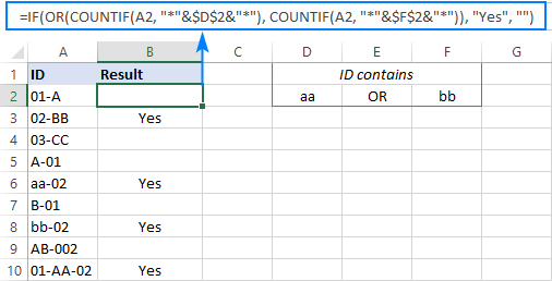
The above formulas work well for 2 partial matches, but if you are searching for 3 or more, they would become too lengthy. In this case, it stands to reason to approach the task differently:
Supply multiple substrings to the SEARCH function in an array constant, count the returned numbers, and check if the result is greater than zero (which would mean that at least one of the substrings if found):
=IF(COUNT(SEARCH({"aa","bb"}, A2))>0, "Yes", "")
This way, you will get exactly the same result with a more compact formula:
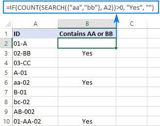
Excel IF AND formula with wildcards
When you want to check if a cell contains two or more different substrings, the easiest way is to use the COUNTIFS function with wildcards for the logical test.
Supposing you want to locate cells in column A that contain both "b" AND "2". To have it done, use "*b*" and "*2*" for COUNTIFS's criteria and A2 for the criteria range:
=IF(COUNTIFS(A2, "*b*", A2, "*2*"), "Yes", "")
Another way is to use the IF AND formula together with ISNUMBER SEARCH:
=IF(AND(ISNUMBER(SEARCH("b", A2)), ISNUMBER(SEARCH("2", A2))), "Yes", "")
Though we do not include any wildcard characters in this formula, it does work like searching for two wildcard strings ("*b*" and "*2*") in the same cell.
Of course, nothing prevents you from entering the search values in predefined cells, D2 and F2 in our case, and supplying the cell references to the formula:
=IF(AND(ISNUMBER(SEARCH($D$2, A2)), ISNUMBER(SEARCH($F$2, A2))), "Yes", "")
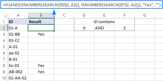
If you prefer using more compact formulas wherever possible, then you may better like the array constant approach. The IF COUNT SEARCH formula is very much like in the previous example, but because this time both substrings must appear in A2, we check if the count is equal to 2:
=IF(COUNT(SEARCH({"b","2"}, A2))=2, "Yes", "")
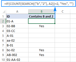
These are the main methods of using wildcard in IF statement in Excel. If you know any other solutions, other users will certainly appreciate if you share your experience in comments. I thank you for reading and hope to see you on our blog next week!
Practice workbook for download
Excel IF wildcard formula examples (.xlsx file)
 by
by
84 comments
You have a lot of great information here.
Could you help me sort out the best way of writing a formula to calculate a value in one cell based a value in another cell. For instance, I am trying to calculate a percent of service utilization based on the type of service that was done. The services are named "BPM, CPM, 500 HR, 500 HR PM, VACUUM TRAILER BPM, AND VACUUM TRAILER CPM. All of the services containing BPM would need to base the calculation on 250, all of the service containing 500 HR would need to base their calculations on 500, and all of the services containing CPM would have to base their calculation on 1000. What I initially wrote was "=IF(D2="*BPM*", Q2=(250-O2)/250, IF(D2="*HR*", Q2=(500-O2)/500, IF(D2="*CPM*", Q2=(1000-O2)/1000,"")))". This came back as a false and left the cell blank but shouldn't have if I wrote it correctly because the referenced cell contains BPM.
Could you tell me where I made the mistake or mistakes?
Hello John!
If you read the article above carefully, you will see that you cannot determine a partial match by this method. Use the method suggested in the article above.
Instead of D2="*BPM*", use COUNTIF(D2,"*BPM*").
For example:
=IF(COUNTIF(D2,"*BPM*"),(250-O2)/250,IF(COUNTIF(D2,"*HR*"),(500-O2)/500,""))
To determine if text strings are a partial match, you can also use these guidelines: How to find substring in Excel
Instead of D2="*BPM*", use ISNUMBER(SEARCH("BPM",D2)).
The formula might look as follows:
=IF(ISNUMBER(SEARCH("BPM",D2)),(250-O2)/250,IF(ISNUMBER(SEARCH("HR",D2)),(500-O2)/500,""))
If you want to write the calculated value in cell Q2, you do not need to specify this cell in the formula. Please read this manual carefully: Nested IF in Excel – formula with multiple conditions.
Thank you! That was what I was missing. I appreciate your assistance and prompt response!
That worked great for the hour based readings because I could search for text to calculate the formula. However, I have multiple conditions for the mileage based service intervals.
For example. I tried =IF(ISNUMBER(SEARCH(6000,D4),(6000-O4)/6000,IF(ISNUMBER(SEARCH(15000,D4),(15000-O4)/15000,IF(ISNUMBER(SEARCH(50000,D4),(50000-O4)/50000,IF(ISNUMBER(SEARCH(5000,D4),(5000-O4)/5000,IF(ISNUMBER(SEARCH(8000,D4),(8000-O4)/8000),IF(ISNUMBER(SEARCH(3500,D4),(3500-O4)/3500),"")))
I also tried CountIF. Both formulas give a window stating " You've entered too many arguments for this function. Is there another function I can use. Did I enter it incorrectly?
D4 in this case contains the mileage based service interval such as "BPM 6000", "CPM 50000", "Brake check/ 15000", "BPM 3500", OR "BPM 8000". O4 will be where it shows the percentage of the service interval utilized so far.
I'm sorry, I mis stated what O4 is. O4 is the miles until due. Q4 is where the formula is input to show the percentage of the service interval utilized so far.
This was soo helpful. I tried so many variations of the SUMIF(S) formula in an attempt to include multiple criteria from the same column in my formula. I eventually came to the thought, can i do a partial match as my data had leading letters and varying numbers. I spent two hours searching the right variation of the IF function! When I was able to apply this solution, I almost broke the desk!! Thank you so much!
i have a address of multiple cities in excel cells consisting around 140 city names, I want to just drag the city name from every cell there are around 10k+ address in a sheet. the address is not in standard format or comma separated. can any one guide.
I just needed a simple formula that allowed using wild cards and IF(Count worked perfectly.
Thank you very much for providing this solution
Hi there,
My problem is the following:
- I have a alphanumerical cell in column A with variable length from 3 digits to 20;
- The alphanumerical code "12ZT" could be present at a fixed location in the string 1 to 4 (e.g. 12ZT5XY39012XY36789 or 12ZT5XY39012XY36789 or 12ZT5XY39012AAA or 12ZT5XY3 or 12ZT556789XY3);
- If the alphanumerical code "12ZT" is present at a fixed location 1 to 4 in the string, the alphanumerical code "XY3" could be present also at a fixed location further in the string 6 to 8 but can also be repeated at a further length location in column A in a random position (e.g., 12345XY39012XY36789 or 12345XY39012AAA or 12345XY39012AXY3 or 12345XY39);
I want to transform the value to another column in the following way:
A B
12ZT5XY39012XY36789 5909012XY36789 (i.e., character in the 5th position after code "12ZT", if "XY3" code exists in the 6 to 8th position all the characters from the 9th position for up to 6 characters on)
12345XY39012AAA 12345X (i.e., no code "12ZT" exists so only up to 6 first characters)
123 123 (i.e., no code "12ZT" exists so only up to 6 first characters)
3210 3210 (i.e., no code "12ZT" exists so only up to 6 first characters)
12345XY39012AXY3 12345X (i.e., no code "12ZT" exists so only up to 6 first characters, XY3 in whatever location is ignored)
12345678XY32 123456 (i.e., no code "12ZT" exists so only up to 6 first characters, XY3 in whatever location is ignored)
21345678XY32 213456 (i.e., no code "12ZT" exists so only up to 6 first characters, XY3 in whatever location is ignored)
IF LEFT Function could be used inside COUNTIF it would be possible (IT IS NOT...), but I see no turnaround:
=IF(LEFT($A1,4)="12ZT",IF(COUNTIF(LEFT($A1,4),"12ZT?XY3")),MID($A1,9,20),MID($A1,5;20)),LEFT($A1,6)
However this doesn't work (the part of LEFT inside a COUNTIF). Any suggestions?
Thanks in advance
Hi! Unfortunately, your explanations are not very clear. For example, the result is 5909012XY36789, 123 123 and 3210 3210. You can identify that "XY3" is in position 6 by using the SEARCH function. For example:
=IFERROR(SEARCH("XY3",A1),0)=6
Please clarify your specific problem or provide additional information to understand what you need.
Hi there - great article. I am looking for a way to drag this formula down an entire column to have the formula search for roughly 10,000 different partial matches in another column. Is there a way to do this? Or would I have to rewrite the formula 10,000 times based on the partial match I am looking for?
Hi! If I understand your task correctly, this guide may be helpful: Copying formula to the entire column.
Hello!
I'm trying to devise a formula that will search for book ISBNs (eg 9780746033168) in cell A1, in another data set where some of the ISBNs have been shortened, removing the first 4 digits. So the matching value would actually be 746033168. I'd like the result to be either 'Not Found' if not found, or 'Partial Found' or similar.
Thank you so much,
Steph
Hi! If I understand your task correctly, this guide may be helpful: How to remove first (left) or last (right) characters in Excel. For example,
REPLACE(A1, 1, 4, "")
or
MID(A1,5,15)
Hello,
I have an excel sheet that has 6000 cities and need to put the state in a separate column. The state is in the original column, but I would like to do some macro research rather than gathering data on individual cities. How do I get the state to auto populate? For example: If my first 3 cells contain Miami, FL, Atlanta, GA and Las Angeles, CA...I would like a text return of FL, GA, CA respectively. What is the best function to have multiple rules in one text return fucntion?
Hi! You can extract the last 2 characters after a space or the last word from the text using these formulas:
=RIGHT(A1,2)
=TEXTAFTER(A1," ")
=TRIM(RIGHT(SUBSTITUTE(A1, " ", REPT(" ", LEN(A1))), LEN(A1)))
Look for the more examples formulas here: Get last word from string.
May I request for help please? I am trying to match data with 2 criterias and return "valid" if true
Criteria 1: Partial Text Match
Criteria 2: Greater than 1
Assuming the following columns:
Column A:
Row 1: Company A
Row 2: Company B
Row 3: Company C
Row 4: Company D
Column B:
Row 1: $100
Row 2: $0
Row 3: $100
Row 4: $-1
Answer:
Row 1: Valid
Row 2: Invalid
Row 3: Valid
Row 4: Invalid
Logic: Company A Match in Name with Greater than 1 Value, that is why the answer is Valid
Thank you
Hope someone can help
I recommend using INDEX & MATCH in conjunction. Here's the written out words of how to set up the formula.
=INDEX(Column where ultimate answer for this cell can be found, MATCH(1,INDEX((cell where first criteria is located=Column where answer to first criteria is located)*(cell where second criteria is located=column where answer to second criteria is located),0,1),0))
I suspect you've already solved your problem though.
Great article. I was trying to use the "Excel IF AND formula with wildcards" piece of your article, but I need to limit the search to just a subset of the string in the cell.
My example.
Trying to search the cases where text string "|Working|Office|" exists but only between two other strings "|Week2|Thursday|Working|Teleworking|" and "|Week2|Friday|Working|Teleworking|"
"Week1|Monday|Working|Teleworking|06:30 AM|03:00 PM|Week1|Tuesday|Working|Teleworking|06:30 AM|03:00 PM|Week1|Wednesday|Working|Teleworking|06:30 AM|03:00 PM|Week1|Thursday|Working|Teleworking|06:00 AM|07:30 AM|Working|Office|09:00 AM|04:00 PM|Week1|Friday|Working|Teleworking|06:30 AM|03:00 PM|Week2|Monday|Working|Teleworking|06:30 AM|03:00 PM|Week2|Tuesday|Working|Teleworking|06:30 AM|03:00 PM|Week2|Wednesday|Working|Teleworking|06:30 AM|03:00 PM|Week2|Thursday|Working|Teleworking|06:00 AM|07:30 AM|Working|Office|09:00 AM|04:00 PM|Week2|Friday|Working|Teleworking|06:30 AM|03:00 PM"
Basically, searching for:
|Week2|Thursday|Working|Teleworking| WILDCARD |Working|Office| WILDCARD |Week2|Friday|Working|Teleworking|
Hi! Use the SEARCH function to find the position of your text strings in the text and compare them.
=IFERROR(SEARCH("|Working|Office|",A2, SEARCH("|Week2|Thursday|Working|Teleworking|",A2)) < SEARCH("|Week2|Friday|Working|Teleworking|",A2),FALSE)
Elegant! Thank you!
I am trying to come up with a formula that takes the value in column P and looks through the entire column L to see if the word in column P is contained in column L. The words are not exact matches. Column L could have the value of "23GAL0163, GASCHEM ARCTIC, 05/" and Column P could have the value of "GASCHEM ARCTIC". Because the word GASCHEM ARTIC is contained in "23GAL0163, GASCHEM ARCTIC, 05/", then I would need it to return the value that is in column P which is "GASCHEM ARCTIC".
Please let me know if you need any further explanation. I really appreciate any and all help!
Hi! To determine if text strings are a partial match, use these guidelines: How to find substring in Excel (partial match). I hope it’ll be helpful. If something is still unclear, please feel free to ask.
Any chance anyone can help me with this? I'm trying to return a 1 for all cells that begin with White but don't include CW or BW. Is this even possible?
=IF(OR(COUNTIF(E2, "White*"),COUNTIF(E2, "*CW*"),COUNTIF(E2,"*BW*")),1,0)
Hi! The formula below will do the trick for you:
=(LEFT(A1,5)="White")*NOT(ISNUMBER(SEARCH("CW",A1)))*NOT(ISNUMBER(SEARCH("BW",A1)))
For more information, please read: How to find substring in Excel
I am trying to create a formula that will check for wildcards and confirm data matches. I have anywhere from 1 to 6 rows where the ID # is the same (Column D) and, in those same rows, I need to know if any of the codes in Column F match the information with wildcard (I put those in S and T 1 cells). If any do, I need it to return either "true" or "Up to Date"(preferred). Because I don't know how many rows for each ID, I tried using an and argument but I'm getting an error I cannot see and I have even written long form in an effort to find it
=IF(($D2=$D8),(countifs(F8=$S$1&"*",F8=$T$1&"*"),"Up to Date",IF(($D2=$D7),(countifs(F7=$S$1&"*",F7=$T$1&"*"),"Up to Date",IF(($D2=$D6),(countifs(F6=$S$1&"*",F6=$T$1&"*"),"Up to Date",IF(($D2=$D5),(countifs(F5=$S$1&"*",F5=$T$1&"*"),"Up to date",IF(($D2=$D4),(countifs(F4=$S$1&"*",F4=$T$1&"*"),"Up to date",IF(($D2=$D3),(countifs(F3=$S$1&"*",F3=$T$1&"*"),"Up to date",IF(($D2=$D2),(countifs(F2=$S$1&"*",F2=$T$1&"*"),"Up to date",""))))))
Any assistance is greatly appreciated!
Hi! I can't check your formula because I don't have your data. Please provide me with an example of the source data and the expected result.
My apologies - It didn't copy before
Cell S1 - CMBI
Cell T1 - CPBI
COL D COL E COL F
00012 Covid Vaccine Dose 1 - Moderna CMOD1
00012 Covid Vaccine Dose 2 - Moderna CMOD2
00012 Covid Vaccine Dose 3 - Moderna CMOD3
00037 Covid Vaccine Dose 1 - Pfizer CPFR1
00037 Covid Vaccine Dose 2 - Pfizer CPFR2
00040 Covid Vaccine Dose 1 - Pfizer CPFR1
00040 Covid Vaccine Dose 2 - Pfizer CPFR2
00044 Covid Vaccine Dose 1 - Pfizer CPFR1
00044 Covid Vaccine Dose 2 - Pfizer CPFR2
00071 Covid Vaccine Dose 1 - Moderna CMOD1
00071 Covid Vaccine Dose 2 - Moderna CMOD2
00071 Covid Vaccine Dose 3 - Moderna CMOD3
00071 Covid Vaccine Dose 4 - Moderna CMOD4
00071 Covid Moderna Bivalent - Dose 5 CMBI5
Only the last line should return a result "up to date", all others should return a blank cell
Thank you again!
Hi! Your data did not help me understand what you want to do. Your formula does not work because it contains an error in the nested IF. I don't know what result you want to get, so I don't have the ability to look it up in such a long formula. Also, countifs(F8=$S$1&"*",F8=$T$1&"*") is incorrect. You can see more information about the COUNTIFS function here: How to use Excel COUNTIFS and COUNTIF with multiple criteria.
Hi!
Can you help me for
=IF(ISNUMBER(SEARCH("III"; ".III.2023."; A2)); "3"; " ")
the number of 3 is month, text "III" is code for month, I will create code "III, IV, and V" for month "3, 4, and 5"
Can you help me please?
i'm sorry if my english so bad :(
Hi! Use a nested IF function or an IFS function for several conditions. For example:
=IF(ISNUMBER(SEARCH("III"; A2)); "3"; IF(ISNUMBER(SEARCH("IV"; A2)); "4"; " "))
=IFS(ISNUMBER(SEARCH("III"; A2)); "3"; ISNUMBER(SEARCH("IV"; A2); "4"))
I don't see your data, but pay attention to the correct use of the SEARCH function.
Hi Alexander
I'm hoping you'll be able to help :)
I am looking for a partial vlookup. And example would be:
In tab 1 it might say; Michelle is bad at excel
In tab 2 it will say: She is not good at excel
I need to do a partial search - and then bring back a row in the 2nd tab (to the first tab) if "excel" (as an example) is in both tabs - Does that make sense? The issue is - "excel" won't be the same in every line (I have about 600 lines) which has somewhat matching info, but slightly different!
Thanks!
Michelle
Hi!
If you want to find a specific word in a cell, try this instruction: How to find substring in Excel (partial match). I hope it’ll be helpful.
Hello all. Fantastic advice here. Hope there is help for this query.
How to write formula to determine if numerical portion/partial text from Column B exists in Column A?
The data in Column B will change so I'm trying to avoid needing to enter it manually.
What I have so far is
=IF(ISNUMBER(SEARCH("110101",A2)),"VALID","INVALID")
The "110101" is the portion I'm stuck on. This value will not always remain the same. Unsure if I'm using the correct formula or need to add a COUNTIF. Any help would be appreciated.
Example of spreadsheet data
Column A Column B
DC-11010101 XM110101
DC-11010102 XM110101
DC-11010103 XM110101
DC-11010201 XM110102
DC-11010202 XM110102
DC-11010203 XM110102
DC-11010301 XM110103
DC-11010302 XM110103
Apologies in advance, but looks like formatting in spreadsheet example didn't come through.
Column A
DC-11010101
DC-11010102
DC-11010103
DC-11010201
DC-11010202
DC-11010203
DC-11010301
DC-11010302
Column B
XM110101
XM110101
XM110101
XM110102
XM110102
XM110102
XM110103
XM110103
Hello!
You are on the right path. Replace the text string in the formula with a reference to the cell that contains the lookup value.
For example,
=IF(ISNUMBER(SEARCH(D2,A2)),"VALID","INVALID")
Hi,
I'm looking for a way to see if a field contains a wildcard match from a list from a different sheet.
So: if field A2 is 'www.website.com/full-url.html' I'd hope to see 'YES' in B2, and for A3 -which is 'www.website-no2.com/url-string.php' - it would return 'NO' in B3, with the other sheet containing the following list:
example.com
websites.com
website.com
another-example.com
I'm aware that the other way around is easier, but I have to match multiple sheets with the same list...
Thanks a lot for your help!
Hello!
To determine partial matches between text strings, use the SEARCH and ISNUMBER functions.
=IF(SUM(--ISNUMBER(SEARCH($D$1:$D$4,A2))),"Yes","No")
Hope this is what you need.
Hi,
I want max partial match formula in excel. Few example given below.
MR. S CHANDRAN - CHANDRAN S = match
MR SAI RATNAKAR KODE - KODE SAI RATNAKAR = match
MR UMESH UMESH ARUN KALE - UMESH ARUN KALE = match
Hi!
This task can be solved using a VBA macro or a special tool. I'd recommend you to have a look at our Fuzzy Duplicate Finder tool that can help you to find partial matches of text strings. It is available as a part of our Ultimate Suite for Excel that you can install in a trial mode and check how it works for free.
Hi, I wonder if you can help me?
I need a formula which will count strings in cells whereby if a particular value appears multiple times within a particular string it will count each occurrence within one cell and for the full row.
Thanks
Hi!
Using the MID function, determine how many times the text from cell D1 is found in the text of cell A1.
=SUM(--(MID(A1,ROW(A1:A100),LEN(D1))=D1))
Hope this is what you need.
Hi, thanks for your speedy response!
Unfortunately this returned a '0' rather than the intended '11'
Perhaps I should have been more clear in the first instance
My data is stored on a second tab within the same workbook, titled 'Data Input', the column of the data which I need the formula to count is titled 'Colour Used?'
The formula is present on another tab called 'Analysis' and the word 'blue' in in cell C40
The data appears as follows, as a string of text within one cell, in column 'U';
Colour Used?
red, yellow, blue, green
red, blue, green
yellow, blue, green
blue, yellow, blue, red, green
green, red, blue
blue, green, yellow
red, blue, green, yellow
yellow
blue, red, yellow, green
yellow, blue, green
pink, yellow, blue, red
I need the formula to count each occurrence of the word 'blue' when it appears more than once within a particular cell, as it does in the 4th cell down, above, total should be '11'.
I have tried the following formula which retuned '0'
=SUM(--(MID('Data Input'!U2,ROW(Table1[Colour Used?]),LEN(C40))=C40))
Any further advice would be greatly appreciated
Many thanks
Hello!
To merge numbers into a string, use the TEXTJOIN function.
=TEXTJOIN("",TRUE,IF(MID(A1,ROW(A1:A200),LEN(D1))=D1,1,""))
Hope this is what you need.
Hi Alexander,
No not that one either, i need to count recurrences of partial text within a cell and a column where that text may appear multiple times,
Currently i can only get it to count the cells whereby it returns and inaccurate value as it is counting the cells rather than the occurrences of text.
Is this possible?
Thanks
Hi!
Copy the first formula down the column and calculate the sum.
Hello, I already read the whole page, and I am amazed of your expertise.
I want to ask you for opinion, as I am struggling with the following requirement.
I need to search for a few substrings at once in the proper column, and based on that to make decision what to replace on those fields as whole value, not replace just the substring. So I need to check which of the x substrings the value belongs to, and based on that, to be replaced in whole column at once.
I tried these queries but they work just for the first cell,not for the whole column. I guess the issue occurs when I put the part "A2:A27".
1.
=IF(COUNT(SEARCH({"substring1", "substring2", "substring3"}, A2:A27)) >0, "some preset day", DATEDIF(some preset date, A2:A27, "d"))
2.
=IF(OR(COUNTIF(A2:A27, "*substring1*"), COUNTIF(A2:A27, "*substring2")), "some preset day", DATEDIF(some preset date, A2:A27, "d"))
Hi,
I'm struggling with matching two worksheets with names ( last name, first name). One worksheet includes names with middle name initials and the other doesn't( it's a large file).
I'm using the formula:
=ISNUMBER(MATCH(A1,Datasource'!$A:$A,0))
A1 = names from worksheet 1 ( names without middle initials)
Datasource = worksheet 2 ( names with middle initials)
I'm getting a true/false result. Some results show "FALSE" even though they should be "TRUE" only because names in sheet 1 don't include middle names.
How can match them partially so worksheet 1 matches worksheet 2?
Please help! Thanks.
Joy
Hello!
To determine partial text matches, you can use the SEARCH function.
If I got you right, the formula below will help you with your task:
=ISNUMBER(MATCH(TRUE,ISNUMBER(SEARCH(A1,Datasource'!A1:A100)),0))
I hope my advice will help you solve your task.
Thank you for your prompt reply.
I tried the formula you provided, and it worked!
Thank you! I greatly appreciate your help!
Joy
Tried many examples of the =IF(ISNUMBER(SEARCH("A", A2)), "Yes", "No") function, but none of them work.
Hi!
Describe the problem in more detail. Perhaps the guide to the SAERCH function will help you.
I've been trying to find a formula that searches a column of postal codes where if the another cell matches on from the column it labels the cell true.
Hi!
If I understood the question correctly, then this article may help - How to compare two columns in Excel for matches and differences. If they don’t work for you, then please describe your task in detail.
EG.
Column A consist of A6123, B4569, C1238, D7895, E1239.
Column B consist data 123 = V1, 456 = V2 , 789 = V3 (lets say we have 100 of these need to match with Column A)
Criterial,
Column A which cell partial consist of 123 or 456 or 789... will prompt as V1 or V2 or V3
Hi!
To find partial text matches, use the SEARCH function. The result of the search is converted to TRUE or FALSE using the ISNUMBER function.
=IF(ISNUMBER(SEARCH($B$1,A1)),"V1", IF(ISNUMBER(SEARCH($B$2,A1)),"V2", IF(ISNUMBER(SEARCH($B$3,A1)),"V3","")))
Hope this is what you need.
=IF(ISNUMBER(SEARCH($B$1,A1)),"V1"...
By any chance i could change $B$1 to refer from a table? EG: =IF(ISNUMBER(SEARCH($B$1:$B$100,A1)) "but this is not working"
Hi!
Before making changes to a formula, read carefully about how the SEARCH function works.
The formula I sent to you was created based on the description you provided in your first request.
Hello,
Thanks for this article. I still have a question: can we replace the *text* i'm looking for by the cell number with * to check in the whole cell if the text appears ?
Thank you
Hi!
I am not sure I fully understand what you mean.
=IF(COUNTIF(AC8, "*Tue*"),"40", ""+COUNTIF(AC8, "*Wed*"),"32.5", ""+COUNTIF(AC8, "*Fri*"),"40", ""+COUNTIF(AC8, "*Sat*"),"48", ""))
Is there another way to rewrite this as excel is not allowing this because there are too many arguments
Hello!
Your formula is wrong. You can find the examples and detailed instructions here: Nested IF in Excel – formula with multiple conditions. I don't know what result you want, but maybe it should look like this:
=IF(COUNTIF(AC8,"*Tue*"),"40",IF(COUNTIF(AC8,"*Wed*"),"32.5",IF(COUNTIF(AC8,"*Fri*"),"40",IF(COUNTIF(AC8,"*Sat*"),"48",""))))
Hi there,
I kindly need help with an If function and wild cards returning different values based on if a job title contains a certain word as below
=IF(C2="*Manager*", 100, IF(C2="*Director*", 100, IF(C2="*Specialist*", 20, 0))).......
Since the F function dosn't work with Wild cards how can i execute this please
Many thanks
Barack
Hello!
To determine the presence of a certain word in the text, instead of C2=”*Manager*” try to use SEARCH function:
ISNUMBER(SEARCH("Manager",C2))
If the word is found it will return TRUE
Great! Will try that. thank you
Can you exclude a character, such as "the second character cannot be an "S" "?
Hello!
To extract the second character from the text, use the MID function.
=MID(A2,2,1) < > "S"
Hello Ablebits, I've been learning a lot and truly benefiting from everything you guys teach here as I love manipulating data within excel. Thank you so much for sharing such useful content!
I wondered if you could help with this one:
I'm working with databases that are not structured. I want to be able to structure them by pulling the strings gfromm the cells (and structure them onto another sheet. eg:
Beautiful convertible white car 2 doors.
4 doors tough black truck
Used gray motorcycle
I want to be able to capture data that are expected, such as color white, gr, type (motorcycle, truck, car) and structure them by placing them into a column /rwow in a different sheet.
Not sure if this is too complicated but If I'm able to capture at least the expected wildcards: motorcycle, car, white etc and place them in different cells would also help me tons!
Any help is really appreciated!
Hello!
To extract color, you can use the formula
=CONCAT(IF(ISNUMBER(SEARCH({"car","truck"},B2,1)), TRIM(MID(SUBSTITUTE(B2," ",REPT(" ",50)), SEARCH("truck", SUBSTITUTE(B2," ",REPT(" ",50)),1)-100,99)),""))
I hope my advice will help you solve your task.
Wow, thanks for your prompt reply Alexander,
Would it be possible to unpack the formula? I try running it but it didn't work...
Hello!
I cannot copy this formula into your workbook. The formula works. What error are you getting?
Thanks for the reply and sorry I wasn't clear, Alexander.
I placed your formula on the B1, and the text "Beautiful convertible white car 2 doors." I placed on cel B2. The error is #VALUE.
The is the scenario:
A1 - Beautiful convertible white car 2 doors.
A2 - 4 doors tough black truck
A3 - Used gray motorcycle
I'd like to be able to format it like:
Car white convertible
truck black 4 doors
motorcycle gray -
The parameters in the column A will be expected such as car, truck, motorcycle, bike, plane, just like the column B and C.
I appreciate your attention and help provided so far,
Hi!
The formula I sent to you was created based on the description you provided in your first request. However, as far as I can see from your second comment, your task is now different from the original one.
The Formula
=CONCAT(IF(ISNUMBER(SEARCH({"car","truck"},B2,1)),TRIM(MID(SUBSTITUTE(B2," ",REPT(" ",50)),SEARCH({"car","truck"},SUBSTITUTE(B2," ",REPT(" ",50)),1)-100,99)),""))
extracts the word that comes before the parameter "car" or "truck".
If you immediately described what you want to receive, I would answer that this is impossible and we would not waste time.
Hello Alexander, thank the reply and sorry for wasting your time.
Unfortunately, the formula hasn't worked. I've got the same #Value message.
Regardless, I appreciate your patience and effort in trying to help...
Great article! I'm wondering if you can expand on the options of the =if(or(countif......
I want different values if true or false. example
=IF(OR(COUNTIF(A2, "*apple*"), "fruit", ""),(COUNTIF(A2, "*lettuce*"), "Veggie", ""),COUNTIF(A2, "*potatoe*"), "root", "") etc
Is this possible?
Thanks!
Hi!
It is possible to use COUNTIF as a condition in an IF function. But you need to write down a condition, not just a formula. For example, COUNTIF(A2, “*apple*”)>3.
I recommend reading this guide: Excel IF statement with multiple AND/OR conditions
Hi thanks for these tutorials
I just wonder instead of marking yes or no I want the opposite cells to be marked as check mark ☑ or X mark but it won't work could it be possible? Thanks though ☺
Hi Cheryl,
For a check mark, you can use CHAR(252) or CHAR(254)
For a cross mark, CHAR(251) or CHAR(253)
Given the above, this formula:
=IF(COUNTIF(A2, "*a*"), "yes", "no")
can be transformed into this one:
=IF(COUNTIF(A2, "*a*"), CHAR(252), CHAR(251))
Note! For the check symbol and cross mark to display correctly, the Wingdings font should be set for the formula cells.
If you are curious to learn more, you may find this tutorial helpful: 6 easy ways to insert a tick symbol and cross mark in Excel
This is a wonderful guide, very detail and well written. Thanks so much!
Great solution. Had to hunt around for this!!
This is a wonderful guide. I am looking for optional responses. Is this possible?
If cell H2 contains "*>AmendCreateTerminate<*" then enter "Terminate" in this cell
Hello
An Excel formula can change the value only in the cell that it is pasted in. If you need to change the content on the cell that has some value in it, you’ll need to use a VBA macro.
How to compare 5 different partial texts each having a specific text value to be entered in my spread sheet. Example: Part text a = text aa
Part text b = text bb.
Part text c = text cc. And so on where text aa, bb, and cc are entered into my cell.
Thank you for your help.
Russ
Hello!
I hope you have studied the recommendations in the tutorial above. It contains answers to your question.
Please specify what you were trying to find, what formula you used and what problem or error occurred. Give an example of the source data and the expected result.
It’ll help me understand it better and find a solution for you.