The tutorial shows how to create multiple IF statements in Excel with AND as well as OR logic. Also, you will learn how to use IF together with other Excel functions.
In the first part of our Excel IF tutorial, we looked at how to construct a simple IF statement with one condition for text, numbers, dates, blanks and non-blanks. For powerful data analysis, however, you may often need to evaluate multiple conditions at a time. The below formula examples will show you the most effective ways to do this.
How to use IF function with multiple conditions
In essence, there are two types of the IF formula with multiple criteria based on the AND / OR logic. Consequently, in the logical test of your IF formula, you should use one of these functions:
- AND function - returns TRUE if all the conditions are met; FALSE otherwise.
- OR function - returns TRUE if any single condition is met; FALSE otherwise.
To better illustrate the point, let's investigate some real-life formulas examples.
Excel IF statement with multiple conditions (AND logic)
The generic formula of Excel IF with two or more conditions is this:
Translated into a human language, the formula says: If condition 1 is true AND condition 2 is true, return value_if_true; else return value_if_false.
Suppose you have a table listing the scores of two tests in columns B and C. To pass the final exam, a student must have both scores greater than 50.
For the logical test, you use the following AND statement: AND(B2>50, C2>50)
If both conditions are true, the formula will return "Pass"; if any condition is false - "Fail".
=IF(AND(B2>50, B2>50), "Pass", "Fail")
Easy, isn't it? The screenshot below proves that our Excel IF /AND formula works right:

In a similar manner, you can use the Excel IF function with multiple text conditions.
For instance, to output "Good" if both B2 and C2 are greater than 50, "Bad" otherwise, the formula is:
=IF(AND(B2="pass", C2="pass"), "Good!", "Bad")
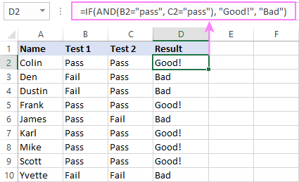
Important note! The AND function checks all the conditions, even if the already tested one(s) evaluated to FALSE. Such behavior is a bit unusual since in most of programming languages, subsequent conditions are not tested if any of the previous tests has returned FALSE.
In practice, a seemingly correct IF statement may result in an error because of this specificity. For example, the below formula would return #DIV/0! ("divide by zero" error) if cell A2 is equal to 0:
=IF(AND(A2<>0, (1/A2)>0.5),"Good", "Bad")
The avoid this, you should use a nested IF function:
=IF(A2<>0, IF((1/A2)>0.5, "Good", "Bad"), "Bad")
For more information, please see IF AND formula in Excel.
Excel IF function with multiple conditions (OR logic)
To do one thing if any condition is met, otherwise do something else, use this combination of the IF and OR functions:
The difference from the IF / AND formula discussed above is that Excel returns TRUE if any of the specified conditions is true.
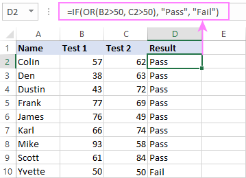
So, if in the previous formula, we use OR instead of AND:
=IF(OR(B2>50, B2>50), "Pass", "Fail")
Then anyone who has more than 50 points in either exam will get "Pass" in column D. With such conditions, our students have a better chance to pass the final exam (Yvette being particularly unlucky failing by just 1 point :)
Tip. In case you are creating a multiple IF statement with text and testing a value in one cell with the OR logic (i.e. a cell can be "this" or "that"), then you can build a more compact formula using an array constant.
For example, to mark a sale as "closed" if cell B2 is either "delivered" or "paid", the formula is:
=IF(OR(B2={"delivered", "paid"}), "Closed", "")
More formula examples can be found in Excel IF OR function.
IF with multiple AND & OR statements
If your task requires evaluating several sets of multiple conditions, you will have to utilize both AND & OR functions at a time.
In our sample table, suppose you have the following criteria for checking the exam results:
- Condition 1: exam1>50 and exam2>50
- Condition 2: exam1>40 and exam2>60
If either of the conditions is met, the final exam is deemed passed.
At first sight, the formula seems a little tricky, but in fact it is not! You just express each of the above conditions as an AND statement and nest them in the OR function (since it's not necessary to meet both conditions, either will suffice):
OR(AND(B2>50, C2>50), AND(B2>40, C2>60)
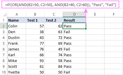
Then, use the OR function for the logical test of IF and supply the desired value_if_true and value_if_false values. As the result, you get the following IF formula with multiple AND / OR conditions:
=IF(OR(AND(B2>50, C2>50), AND(B2>40, C2>60), "Pass", "Fail")
The screenshot below indicates that we've done the formula right:
Naturally, you are not limited to using only two AND/OR functions in your IF formulas. You can use as many of them as your business logic requires, provided that:
- In Excel 2007 and higher, you have no more than 255 arguments, and the total length of the IF formula does not exceed 8,192 characters.
- In Excel 2003 and lower, there are no more than 30 arguments, and the total length of your IF formula does not exceed 1,024 characters.
Nested IF statement to check multiple logical tests
If you want to evaluate multiple logical tests within a single formula, then you can nest several functions one into another. Such functions are called nested IF functions. They prove particularly useful when you wish to return different values depending on the logical tests' results.
Here's a typical example: suppose you want to qualify the students' achievements as "Good", "Satisfactory" and "Poor" based on the following scores:
- Good: 60 or more (>=60)
- Satisfactory: between 40 and 60 (>40 and <60)
- Poor: 40 or less (<=40)
Before writing a formula, consider the order of functions you are going to nest. Excel will evaluate the logical tests in the order they appear in the formula. Once a condition evaluates to TRUE, the subsequent conditions are not tested, meaning the formula stops after the first TRUE result.
In our case, the functions are arranged from largest to smallest:
=IF(B2>=60, "Good", IF(B2>40, "Satisfactory", "Poor"))
Naturally, you can nest more functions if needed (up to 64 in modern versions).

For more information, please see How to use multiple nested IF statements in Excel.
Excel IF array formula with multiple conditions
Another way to get an Excel IF to test multiple conditions is by using an array formula.
To evaluate conditions with the AND logic, use the asterisk:
To test conditions with the OR logic, use the plus sign:
To complete an array formula correctly, press the Ctrl + Shift + Enter keys together. In Excel 365 and Excel 2021, this also works as a regular formula due to support for dynamic arrays.
For example, to get "Pass" if both B2 and C2 are greater than 50, the formula is:
=IF((B2>50) * (C2>50), "Pass", "Fail")

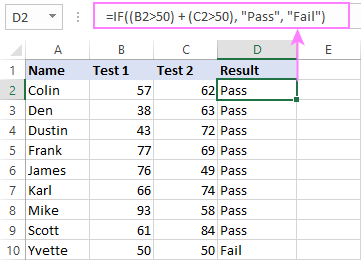
In my Excel 365, a normal formula works just fine (as you can see in the screenshots above). In Excel 2019 and lower, remember to make it an array formula by using the Ctrl + Shift + Enter shortcut.
To evaluate multiple conditions with the OR logic, the formula is:
=IF((B2>50) + (C2>50), "Pass", "Fail")
Using IF together with other functions
This section explains how to use IF in combination with other Excel functions and what benefits this gives to you.
Example 1. If #N/A error in VLOOKUP
When VLOOKUP or other lookup function cannot find something, it returns a #N/A error. To make your tables look nicer, you can return zero, blank, or specific text if #N/A. For this, use this generic formula:
For example:
If #N/A return 0:
If the lookup value in E1 is not found, the formula returns zero.
=IF(ISNA(VLOOKUP(E1, A2:B10, 2,FALSE )), 0, VLOOKUP(E1, A2:B10, 2, FALSE))
If #N/A return blank:
If the lookup value is not found, the formula returns nothing (an empty string).
=IF(ISNA(VLOOKUP(E1, A2:B10, 2,FALSE )), "", VLOOKUP(E1, A2:B10, 2, FALSE))
If #N/A return certain text:
If the lookup value is not found, the formula returns specific text.
=IF(ISNA(VLOOKUP(E1, A2:B10, 2,FALSE )), "Not found", VLOOKUP(E1, A2:B10, 2, FALSE))

For more formula examples, please see VLOOKUP with IF statement in Excel.
Example 2. IF with SUM, AVERAGE, MIN and MAX functions
To sum cell values based on certain criteria, Excel provides the SUMIF and SUMIFS functions.
In some situations, your business logic may require including the SUM function in the logical test of IF. For example, to return different text labels depending on the sum of the values in B2 and C2, the formula is:
=IF(SUM(B2:C2)>130, "Good", IF(SUM(B2:C2)>110, "Satisfactory", "Poor"))
If the sum is greater than 130, the result is "good"; if greater than 110 – "satisfactory', if 110 or lower – "poor".
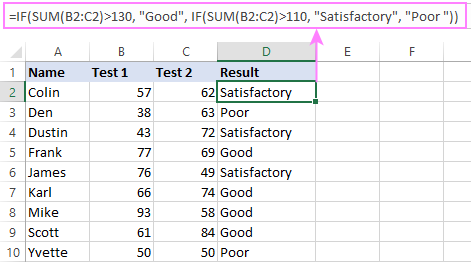
In a similar fashion, you can embed the AVERAGE function in the logical test of IF and return different labels based on the average score:
=IF(AVERAGE(B2:C2)>65, "Good", IF(AVERAGE(B2:C2)>55, "Satisfactory", "Poor"))
Assuming the total score is in column D, you can identify the highest and lowest values with the help of the MAX and MIN functions:
=IF(D2=MAX($D$2:$D$10), "Best result", "")
=IF(D2=MAX($D$2:$D$10), "Best result", "")
To have both labels in one column, nest the above functions one into another:
=IF(D2=MAX($D$2:$D$10), "Best result", IF(D2=MIN($D$2:$D$10), "Worst result", ""))

Likewise, you can use IF together with your custom functions. For example, you can combine it with GetCellColor or GetCellFontColor to return different results based on a cell color.
In addition, Excel provides a number of functions to calculate data based on conditions. For detailed formula examples, please check out the following tutorials:
Example 3. IF with ISNUMBER, ISTEXT and ISBLANK
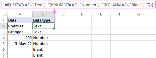
To identify text, numbers and blank cells, Microsoft Excel provides special functions such as ISTEXT, ISNUMBER and ISBLANK. By placing them in the logical tests of three nested IF statements, you can identify all different data types in one go:
=IF(ISTEXT(A2), "Text", IF(ISNUMBER(A2), "Number", IF(ISBLANK(A2), "Blank", "")))
Example 4. IF and CONCATENATE
To output the result of IF and some text into one cell, use the CONCATENATE or CONCAT (in Excel 2016 - 365) and IF functions together. For example:
=CONCATENATE("You performed ", IF(B1>100,"fantastic!", IF(B1>50, "well", "poor")))
=CONCAT("You performed ", IF(B1>100,"fantastic!", IF(B1>50, "well", "poor")))
Looking at the screenshot below, you'll hardly need any explanation of what the formula does:

IF ISERROR / ISNA formula in Excel
The modern versions of Excel have special functions to trap errors and replace them with another calculation or predefined value - IFERROR (in Excel 2007 and later) and IFNA (in Excel 2013 and later). In earlier Excel versions, you can use the IF ISERROR and IF ISNA combinations instead.
The difference is that IFERROR and ISERROR handle all possible Excel errors, including #VALUE!, #N/A, #NAME?, #REF!, #NUM!, #DIV/0!, and #NULL!. While IFNA and ISNA specialize solely in #N/A errors.
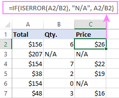
For example, to replace the "divide by zero" error (#DIV/0!) with your custom text, you can use the following formula:
=IF(ISERROR(A2/B2), "N/A", A2/B2)
And that's all I have to say about using the IF function in Excel. I thank you for reading and hope to see you on our blog next week!
Practice workbook for download
Excel IF multiple criteria - examples (.xlsx file)
 by
by
4506 comments
hi I need help for the following
BIO Scheme above 35
Maths Scheme above 40
Technology scheme above 45
Arts Scheme above 55
Hi,
I'm looking for help with a formula:
=IFERROR(IF(H9>90%,H9*G9,"-")
H9 is the % Accomplished, G9 is the Value. The problem I am having is I need the % accomplished to max out at 100%
Thanks
its related to end of service calculation
as per our policy, first 5 years of service, gratuity will be 1 month for each year( ie 30 days X 5) and next 5 years, it is 1.5 month (5and remaining service period it is 2 months.
what should be formula which will check 4 year service, 8 year service and 12 year service.
kindly help me.
thanks
Hi Krishna,
Based on the information provided in your post I give below the formula which should work for you:
A B C D
2 Years worked Months earned
3 6 6.5
4 Cross check calculation
5 Year split Entitled Months
6 5 1 5
7 1 1.5 1.5
8 0 2 0
9 Total 6.5
IF(B25,IF(B210,(5*1)+(5*1.5)+(B2-10)*2,0))))
Let me know if this worked for you,
Regards,
Ramki
Hi Esther,
If you are looking for a match of percentage ranges and the matching values then a lookup table and Vlookup formula can solve your requirement. I can send you the file with the formula and the information I think you are working with.
Hi. Need help for the following.
Above 90% 0
Below 90% to 87% 200
Below 87% to 85% 400
Below 85% to 83% 600
Below 83% 1,200
This does not work (M11 = Result)
=IF(AND(M11>=87%,M11=85%,M11=83%,M11<=85%),K11,IF(AND(M1190%,"")))))
I need help in formulating a complicated IF statement.
So I want a spreadsheet that has one cell that will calculate the correct percentage that is marked with an "X". (However there are five different percentage choices that can be marked are 2%,3%,4%,5% and 6%.)
I started the following Nested IF formula but I'm screwing it up, maybe I need to use an IF/OR formula but can you please help me?
=IF(E4="X",(D4*0.02),0,IF(F4="X",(D4*0.03),0,IF(G4="X",(D4*0.04),0,IF(H4="X",(D4*.05),0,if(G4="X",(D4*.06))))
Hi Gabriel,
I think a nested If formula is the right approach. Try this one:
=IF(E4="X", D4*0.02, IF(F4="X", D4*0.03, IF(G4="X", D4*0.04, IF(H4="X", D4*0.05, IF(G4="X", D4*0.06, "")))))
Hi, Just need some help in creating the formulas for these conditions. Hope you can help me.
If Taxable Income is: Tax Due is:
Not over 10,000 5%
Over 10,000 but not over 30,000 500 + 10% of the excess over 10,000
Over 30,000 but not over 70,000 2,500 + 15% of the excess over 30,000
Hi Rebecca,
Try the following nested If's:
=IF(A1>4999, A1*15%, IF(A1>2999, A1*12%, IF(A1>594, A1*10%, "")))
Thank you so much for your help!
I'm trying to work on a formula for my new employer but I keep getting an error message. Here is what I need it to do:
If A1 = $595 thru $2999 multiply by 10%, but if it = $3000 thru $4999 then multiply by 12%, but if it = greater than $5000 then multiply by 15%.
Please help! Getting frustrated trying. TIA
Hi,
Please advise if I can use the if condition in vlookup. I want to pull data from reference 3, reference 1 and 2 is blank.
Please advise.
Regards,
Arvind
i have a question regarding the first example: IF/AND formula: =IF((AND(C2>=20, D2>=30)), "Pass", "Fail")
Does the order in the "AND" segment matter? I.E. if it was IF((AND(D2>=30, C2>=20)), "Pass", "Fail"), would that change the result?
Hi Kevin,
The order of arguments in AND and OR statements does not matter at all. You can put them in any order and the result will be the same.
Hi, I want to achieve a dollar value and I have created this =IF(F9>2888, "100", IF(F9>1588, "50")). But I have getting 50 and 100 as a text even I try to convert it into number.
Can help?
Hi Kerine,
The point is that Excel interprets any value enclosed in double quotes as a text value. So, simply remove the double quotes surrounding 100 and 50, and your formula will work fine:
=IF(F9>2888, 100, IF(F9>1588, 50))
Thank you so very much for this very helpful / educational posts Ms. Cheusheva.
I want to use If A1 = "82041100 / 82041200 / 82042000" and A2 = "China" then A3 = 150 otherwise 200. Could any one tell me what would be the syntax of the that formula in excel.
Hi Muddassir,
If you mean A1 contains exactly that text string, use this formula:
=IF(AND(A1="82041100 / 82041200 / 82042000", A2="China"), 150, 200)
If you mean A1 contains any of those 3 numbers, use this one:
=IF(AND(OR(A1=82041100, A1=82041200, A1=82042000), A2="China"), 150, 200)
Sorry i have redo this
Hi i want to achieve this, Results should be in D5
Can anyone help me out. Both conditions has to be met.
if C8 68%>= 74.99% Results in Cell D5=200 if C8 >=75%, D5=300
AND
if C9 68%>=75% , then D5=300
if C8 and C9 <68% then D5=0.00
Hi i want to achieve this, Results should be D5
Can anyone help me out. Both conditions has to be met.
C8 68 between 74.99 Results D=200 if C8 >=75%, D=300
AND
C9 68%>==75% , D=300
if C8 and C9 <68% then D=0.00
Hello,
I am trying to write a IF function in excel but not successful :(
I want to write a formula for percentage calculation IF the column is an integer. No percentage calculation if the column zero and not an integer.
Hope to receive your reply. Thanks.
Hi Terrance,
You can use a formula similar to this (just replace A1*10% with the percentage calculation you want):
=IF(AND(A1<>0, INT(A1)=A1), A1*10%, "")
Hi there.
I would like to request how to make a formula for our delivery timeline using the following conditions for Orders made on weekdays, weekends and cutoff time (for weekday orders).
Scenario A
Condition 1: Delivery Address - Provincial
Condition 2: Order Date: Weekday
Condition 3: Order time is before 3PM
Action: Add 5 days to the order date excluding weekends
Scenario B
Condition 1: Delivery Address - Provincial
Condition 2: Order date: Weekend
Condition 3: Order time (N/A)
Action: Add 4 days from Monday= friday
Thanks
It has been very helpful for me and thank you.
If there is word "No" in column A, word #N/A in column B and word "No" in column C, i want the formula so that output is "No" or else it should be "Yes"
Hi,
I want to use the following function, can I?
IF(A1=0;B2=A1*S3;B2=A8*S6)
Regards,
Hi Shaher,
If you are writing a formula for B2, you don't need to reference it in the formula:
=IF(A1=0; A1*S3; A8*S6)
Hi Svetlana,
This is very useful. Appreciate your effort. Cheers!! :)
I am looking for an if, and statement the uses vlookup. I keep getting an error but can't figure it out. I want all 3 conditions to be true to give a 1 if they are in the cell. If not then use the cell in another cell on another tab. This is what I have:
=IF(AND(B48="7R",O48="No Repair Program",vlookup(a48,'Att. A-G'!$A$10:$bj$48,62=0),1,VLOOKUP(A48,'Att. D NIIN DATA'!$A$12:$AG$56,14,FALSE)))
i have problem in IF condition in Excel. B1 is drop down i select one value the automatically how to change in B2. like this........
B1=dropdown 1,2,3
B2=values like 1=6.2
2=5.6
3=6.6
how can do this problem please tel me or send answer my mail
thanking you
=IF(H17=1,6.2,IF(H17=2,5.6,IF(H17=3,6.6)))
thank you
i have small problem in excel. it is i am created a drop down in the excel. like this Ex: B is 1,2,3,4,5.... and C is 45,56,59,58,26..
but iam select B1 then automatically C Cell become changed into 45.
how is it please solve my problem. thanking you
=IF(N15=4,0%))))
I wrote the formula above, but it is returning "False" insteady of an actual number, anybody can help to identify how I can correct this?
this formula was treated =0 why because u r typing in cell N15 some other vales give like 3 or 10. that is not correct vales. the correct vale is only 4. but why u r give IF condition like Cell N15=0% after give in cell N15.
=IF(N15=4,0%)
Hi,
Here is my formula. its not working.
=IF(AND(AR2>=0.9, AR2<=0.7), "C", IF(AND(AR2=0.5), "B",IF(AND(AR2=0.1), "A", "D")))
I am setting up KPI metrics, so based on the data, i have named each value in categories.
If X is between 0.9 to 0.7 = C,0.6 to 0.5=B, 0.4 to 0.1=A, then if is over 0.9=D
Hi
Sri
=IF(AR2>0.9,"D",IF(AR2<=0.4,"A",IF(AR2<=0.6,"B",IF(AR2<=0.9,"C"))))
Regards
Manish
Thanks, these examples are very helpful
$125/100 people or part thereof
I used the following formula:
=B19*IF(B4>100,IF(B4>200,IF(B4>300,IF(B4>400,IF(B4>500,6,5),4),3),2),1)
Is there is a better method or function that could be used?
Also for, requires 1 person per 50 tickets sold, minimum of 5 security personnel at an event. Evening events are charged a flat rate of $200/security person.
I used,
=B21*IF(B4>250,IF(B4>300,IF(B4>350,IF(B4>400,IF(B4>450,IF(B4>500,11,10),9),8),7),6),5)
F347874 is 30-Jun-14
why this formula is showing false
IF(AND(F347874>"03-31-2014",F347874<="09-30-2014")
Please help
All data is in descriptive form .
I tried one formula for counting no entries but it won't work.
=count(if(C1=Sheet1C2),C2:C60)
I need an IF formula to reflect this information:
If cell A1 equals:
Weighted % Points
20%+=3
10.1-20%=2
5.1-10%=1
0-5%=0
IF(A1<5%,0,IF(A1<=10%,1,IF(A1<=20%,2,3)))
I think I have a simple request but have been unable to figure this out.
Cell A1 is used for a price to be input.
Cell B1 needs to output a fee based on the price input into cell A1
The parameters would be as follows:
In A1 $1999 and below should equal $125 in B1
In A1 $2000-$4999 should equal $225 in B1
$4999 and greater should equal A1*.05
Ive tried IF, AND, & OR functions and I can't get it. Please help.
Hi Terrence,
You can use the following nested IF's:
=IF(A1>4999, A1*0.05, IF(A1>1999, 225, 125))
Thanks!
Hi,
I'm a little stuck and I'm hoping I'm trying to use the right formula!
I'm making a document to manage when our contractors are working and our margin.
I need a formula that will work out our margin based on if they are getting paid daily or hourly, thus is cell C35 says Daily I need it to multiply D35 (The margin) by 5, and if it says Hourly it needs to multiply D35 by 37.5.
Thanks in advanced!
Abbie
HI
I'm trying to have an one cell answer (A1) that takes IF from multiple columns. If B1 is 1 then write "Apple", if it's empty, don't write anything. If C1 is 1 then write "Banana", (if empty don't write anything). If D1 is 1 then give "Orange"....
If say B1 and C1 have "1" then the cell should give Apple, Banana.
Many thanks in advance
Diana
Hello,
I'm trying to create a series of columns, the number of which rely upon a set period of time entered by the user (Each represents a week). The date for one column relies on the date of the previous:
=IF(PREVIOUS COLUMN+7 <= END DATE, PREVIOUS COLUMN+7,"")
However this condition causes #VALUE! errors after the last column, so I tried to use the IFERROR function:
=IFERROR(IF(PREVIOUS COLUMN+7 <= END DATE, PREVIOUS COLUMN+7,""),""
as a part of conditional formatting to hide the #VALUE!, but the #VALUE! still keeps popping up. Any advice?
Hi Svetlana,
Can you use 3 rules in a formula?
IF(AND(F20<=99,G14<=29999,J187"28-34 Degree Pitch")"$65.00"
How can I make this formula working, using 3 scenarios.
Really hoping you can assist Svetlana,
I am stuck! I have tried all the formulas I could find on conditional formatting to try to get the following result:
If C2<10 and W2=0 Fill background Red
Hope someone can help:)
Heather,
Go to the cell C2 or W2 you want the the conditional formatting to occur.
Click on the Conditional Formatting Icon and select Manage Rule. You will see a pop-up window the Conditional Formatting Rule Manager.
Click New Rule.. and select "Use a formula to determine which cells to Format" on the Rule Type.
On the empty line "Format values where this formula is true:" enter the formula =c2<10 or click the box on the end of the line which will allow you to pick the cell C2.
Now select the "Format.." button and there are tabs "Number", "Font", "Border" and "Fill". Select the "Fill" tab and under the "Background Color: select the Red color and the Sample window should show red. Click "O.K" to finish up.
Once you type numbers on the cell the formatting should occur if the condition is true then the cell will highlight red.
Hope this helps.
Hi Svetlana,
I am trying to convert marks to grades and it worked using the below formula:
=IF(D2<50,"F",IF(D2<60,"P",IF(D2<70,"D",IF(D2<80,"C",IF(D2<90,"B",IF(D2) instead of (<) and keep the rest exactly the same.. except a trick with the IF he said!!... is there something like this? different function than the IF?? I am confused.
Thanks,
Bas
Hi Svetlana,
I am trying to convert marks to grades and it worked using the below formula:
=IF(E9<50,"F",IF(E9<60,"P",IF(E9<70,"D",IF(E9<80,"C",IF(E9<90,"B",IF(E9 (not <) and keep the rest exactly the same.. except a trick with the IF... is there something like this? different function than the IF?? I am confused.
Thanks,
Bas
Privet Svetlana, ty voobshe genie!
I need the formula for S9 to give me either "Dog", "Top Seller", "Workhorse" or "Challenge".
For eg.:
If P9 = "Low" and R9 = "Low" I need "Dog" in S9
If P9 = "High" and R9 = "High" I need "Top Seller" in S9
If P9 = "Low" and R9 = "High" I need "Workhorse" in S9
If P9 = "High" and R9 = "Low" I need "Challenge" in S9
I hope you can help on that..
Hi Ivan,
Don't think I am, but thanks anyway:)
This can be done by using nested IF's with embedded AND statements, like this:
=IF(AND(P9="low", R9="low"), "dog", IF(AND(P9="high", R9="high"), "top seller", IF(AND(P9="low", R9="high"), "Workhorse", IF(AND(P9="high", R9="low"), "Challenge", ""))))
Please note, if you use Russian of European localization of Office, you may need to replace commas with semicolons in the formula (depending on which List Separator is set in your Regional Settings).
Thanks so much! Problem solved
Удачи
Hello,
Beginner here..I am trying to get a range of cells containing text and display only the most severe result.
My formula that works for only 2 results:
=IF(COUNTIF(F5:F10,"Not OK")>0, "Not OK", "OK")
what i am trying to do is add a "Ok But" text result.
So if there is at least one "Not Ok" with multiple "Ok Buts" the result should be "Not Ok"
If i have at least one "Ok But", no "Not Ok", i need it to show "Ok But"
If all are Ok it should result "Ok"
Thanks
Nevermind,
=IF(COUNTIF(F5:F10, "not ok")>0,"Not Ok",IF(COUNTIF(F5:F10, "Ok But")>0,"Ok But","Ok"))
How can I make a formula to test two different conditions?
For the first condition there are 8 different outcomes.
For the second condition there are 4 different outcomes, however for this one the outcomes are in range of numbers.
ex: 0-1000 = outcome A or 1001-1000=result B
Suppose I get result X for first condition
and for second I get result B however this result needs to be defined by a range of numbers that is directly related to result X.
Ex. Ranges:
00-10 = A
11-20 = B
21-30 = C
31-40 = D
and
there's another variable that changes each level.
variable x
so the above ranges are true if X = 1
however if x=2 then
ranges change for A-D
How can I write a formula to that will tell me the range letter (A-D) if the range changes depending on variable x?
Update.
Russes answer in the comments gave me what I needed.
I was able to nest 32 if statements!
Does anyone know how to define a function in Excel?
Ex. I want:
Weekly = 52
Biweekly=26
Monthly=12
Everything else (literally)=1
Is this possible in excel?
I mean variable not function.
I still don't know who to do if for a range
can you please explain
Like if 300-400 then 1
if 200-299 then 2
if 100- 199 then 3
if < 100 then 4
How can I do that, thanks
hi i need to get this: if between -10 and 5= 5 if between -15 and 10= 4, if between -25 and 15=3, if between -35 and 25=2 and if btween -45 and 35= 1 im having trouble i can use IF and AND but i just get 5 and 4.
please help
these are the formulas i've use
=IF(AND(H6>=-10,H6<=5),"5","4")
=IF(H57=6,"4",IF(H57>15,"3",IF(H57=25,"2","0")))))
Hi Mike,
The point is that your conditions are not mutually exclusive, and lots of numbers fell into all of the categories. For example, number 1 is between -10 and 5, but it is also between -35 and 25, and so on.
In nested functions, Excel checks the conditions in the order they appear in a formula, and if a condition is met, subsequent conditions are not checked. So, I'd advise you either reconsider the logic, or input the conditions in the order of importance.
Hi programmers!
Good day!
I need your program expertise in excel for the ff:
if the program detect the below given Integers (1,2,etc...) it will show the corresponding value (see values).
1 = Approved - May Proceed (Re-Submission Required)
2 = Approved With Comment
3 = Not Approved / Rejected
7 = See Remarks
8 = For Retention
10 = Approved (Re-Submission not Required)
12 = No Comment
AFC = Approved for Construction
AWH = Approved with Comment
Thank you for your respond..
Please help:
Employee subgroup:: MR/Grade 1
• Area I (Jabotabek, Surabaya, Denpasar, Sulawesi, Pekanbaru, Tanjung Pinang, and Riau): IDR 420,000 / month
• Area II (All others except Area I and III: Bandar Lampung, Bandung, Bogor, Cirebon, Jambi, Yogyakarta, Malang, Medan, Padang, Palembang, Solo): IDR 360,000 / month
• Area III (Kalimantan, Batam): IDR 450,000 / month
Employee subgroup: FLSM/Grade 2
• Area I (Jabotabek, Surabaya, Denpasar, Sulawesi, Pekanbaru, Tanjung Pinang, and Riau): IDR 540,000 / month
• Area II (All others except Area I and III: Bandar Lampung, Bandung, Bogor, Cirebon, Jambi, Yogyakarta, Malang, Medan, Padang, Palembang, Solo): IDR 500,000 / month
• Area III (Kalimantan, Batam): IDR 600,000 / month
I want to use the if function but I can't include the employee subgroup.
this was my current formula:
Employee subgroup:: MR/Grade 1
=IF(G17="Area 1", "420,000", IF(G17="Area 2", "360,000", IF(G17="Area 3", "450,000", "")))
Employee subgroup: FLSM/Grade 2
=IF(G33="Area 1", "540,000", IF(G33="Area 2", "500,000", IF(G33="Area 3", "600,000", "")))
That's why, I need to separate the employee subgroups into 2 sheets instead of combining them.
Hi,
I need to create an IF/AND formula based on the information below.
FOR EXAMPLE:
If Cell 'A2' = Very Low & Cell 'B2' = Very Low......then I want Cell 'C2'= 2 (and vice versa)
If Cell 'A3' = "Very High" & Cell 'B3'= Very High.....then Cell 'C3'= 4
(and vice versa)
If Cell 'A4' = Very High & Cell 'B4'= Very Low......then Cell 'C4'= 3
(and vice versa)
So far my formula is =IF((AND(A2="Very Low",B2="Very Low")), "2").....
Please help on how to complete the formula to include the other possible variations
I am having difficulties with the below formula.
=IF(A10&C10&D10="Corrugated & Trimdeck .42 Colorbond Re-roofing"&"28-34 Degree Pitch"&"<=99",E34,)
In this specific example:
A10 = Corrugated & Trimdeck .42 Colorbond Re-roofing
C10 = 28-34 Degree Pitch
D10 = the figure entered is anywhere between 0 and 99
E34 = a cost of $10 should be returned as entered in E34
It does not return the number as detailed in E34, only a 0.
Can I have 3 rules in the one formula?
Hi there, I was wondering if someone could please help with a formula I am trying to put together.
I have sent an e-mail with sample data on support@ablebits.com
I have some text in Column A (around 8,000 rows) and I would like to shortlist that into 10 categories. I am not sure if its possible to put a "If" formula if there was one because of complications around the formatting in Column A.
Can you please help or suggest a way to do this more efficiently as this would be my monthly process.
Thanks in anticipation.