The tutorial shows how to create multiple IF statements in Excel with AND as well as OR logic. Also, you will learn how to use IF together with other Excel functions.
In the first part of our Excel IF tutorial, we looked at how to construct a simple IF statement with one condition for text, numbers, dates, blanks and non-blanks. For powerful data analysis, however, you may often need to evaluate multiple conditions at a time. The below formula examples will show you the most effective ways to do this.
How to use IF function with multiple conditions
In essence, there are two types of the IF formula with multiple criteria based on the AND / OR logic. Consequently, in the logical test of your IF formula, you should use one of these functions:
- AND function - returns TRUE if all the conditions are met; FALSE otherwise.
- OR function - returns TRUE if any single condition is met; FALSE otherwise.
To better illustrate the point, let's investigate some real-life formulas examples.
Excel IF statement with multiple conditions (AND logic)
The generic formula of Excel IF with two or more conditions is this:
Translated into a human language, the formula says: If condition 1 is true AND condition 2 is true, return value_if_true; else return value_if_false.
Suppose you have a table listing the scores of two tests in columns B and C. To pass the final exam, a student must have both scores greater than 50.
For the logical test, you use the following AND statement: AND(B2>50, C2>50)
If both conditions are true, the formula will return "Pass"; if any condition is false - "Fail".
=IF(AND(B2>50, B2>50), "Pass", "Fail")
Easy, isn't it? The screenshot below proves that our Excel IF /AND formula works right:

In a similar manner, you can use the Excel IF function with multiple text conditions.
For instance, to output "Good" if both B2 and C2 are greater than 50, "Bad" otherwise, the formula is:
=IF(AND(B2="pass", C2="pass"), "Good!", "Bad")
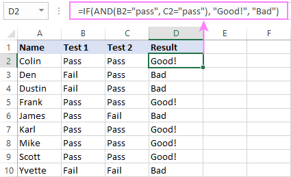
Important note! The AND function checks all the conditions, even if the already tested one(s) evaluated to FALSE. Such behavior is a bit unusual since in most of programming languages, subsequent conditions are not tested if any of the previous tests has returned FALSE.
In practice, a seemingly correct IF statement may result in an error because of this specificity. For example, the below formula would return #DIV/0! ("divide by zero" error) if cell A2 is equal to 0:
=IF(AND(A2<>0, (1/A2)>0.5),"Good", "Bad")
The avoid this, you should use a nested IF function:
=IF(A2<>0, IF((1/A2)>0.5, "Good", "Bad"), "Bad")
For more information, please see IF AND formula in Excel.
Excel IF function with multiple conditions (OR logic)
To do one thing if any condition is met, otherwise do something else, use this combination of the IF and OR functions:
The difference from the IF / AND formula discussed above is that Excel returns TRUE if any of the specified conditions is true.
So, if in the previous formula, we use OR instead of AND:
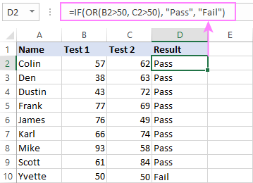
=IF(OR(B2>50, B2>50), "Pass", "Fail")
Then anyone who has more than 50 points in either exam will get "Pass" in column D. With such conditions, our students have a better chance to pass the final exam (Yvette being particularly unlucky failing by just 1 point :)
Tip. In case you are creating a multiple IF statement with text and testing a value in one cell with the OR logic (i.e. a cell can be "this" or "that"), then you can build a more compact formula using an array constant.
For example, to mark a sale as "closed" if cell B2 is either "delivered" or "paid", the formula is:
=IF(OR(B2={"delivered", "paid"}), "Closed", "")
More formula examples can be found in Excel IF OR function.
IF with multiple AND & OR statements
If your task requires evaluating several sets of multiple conditions, you will have to utilize both AND & OR functions at a time.
In our sample table, suppose you have the following criteria for checking the exam results:
- Condition 1: exam1>50 and exam2>50
- Condition 2: exam1>40 and exam2>60
If either of the conditions is met, the final exam is deemed passed.
At first sight, the formula seems a little tricky, but in fact it is not! You just express each of the above conditions as an AND statement and nest them in the OR function (since it's not necessary to meet both conditions, either will suffice):
OR(AND(B2>50, C2>50), AND(B2>40, C2>60)
Then, use the OR function for the logical test of IF and supply the desired value_if_true and value_if_false values. As the result, you get the following IF formula with multiple AND / OR conditions:
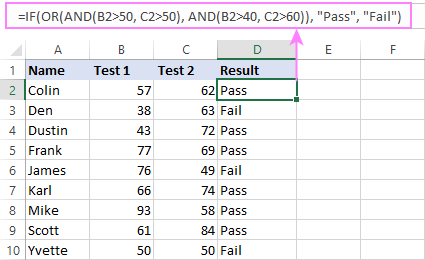
=IF(OR(AND(B2>50, C2>50), AND(B2>40, C2>60), "Pass", "Fail")
The screenshot below indicates that we've done the formula right:
Naturally, you are not limited to using only two AND/OR functions in your IF formulas. You can use as many of them as your business logic requires, provided that:
- In Excel 2007 and higher, you have no more than 255 arguments, and the total length of the IF formula does not exceed 8,192 characters.
- In Excel 2003 and lower, there are no more than 30 arguments, and the total length of your IF formula does not exceed 1,024 characters.
Nested IF statement to check multiple logical tests
If you want to evaluate multiple logical tests within a single formula, then you can nest several functions one into another. Such functions are called nested IF functions. They prove particularly useful when you wish to return different values depending on the logical tests' results.
Here's a typical example: suppose you want to qualify the students' achievements as "Good", "Satisfactory" and "Poor" based on the following scores:
- Good: 60 or more (>=60)
- Satisfactory: between 40 and 60 (>40 and <60)
- Poor: 40 or less (<=40)
Before writing a formula, consider the order of functions you are going to nest. Excel will evaluate the logical tests in the order they appear in the formula. Once a condition evaluates to TRUE, the subsequent conditions are not tested, meaning the formula stops after the first TRUE result.
In our case, the functions are arranged from largest to smallest:
=IF(B2>=60, "Good", IF(B2>40, "Satisfactory", "Poor"))
Naturally, you can nest more functions if needed (up to 64 in modern versions).

For more information, please see How to use multiple nested IF statements in Excel.
Excel IF array formula with multiple conditions
Another way to get an Excel IF to test multiple conditions is by using an array formula.
To evaluate conditions with the AND logic, use the asterisk:
To test conditions with the OR logic, use the plus sign:
To complete an array formula correctly, press the Ctrl + Shift + Enter keys together. In Excel 365 and Excel 2021, this also works as a regular formula due to support for dynamic arrays.
For example, to get "Pass" if both B2 and C2 are greater than 50, the formula is:
=IF((B2>50) * (C2>50), "Pass", "Fail")

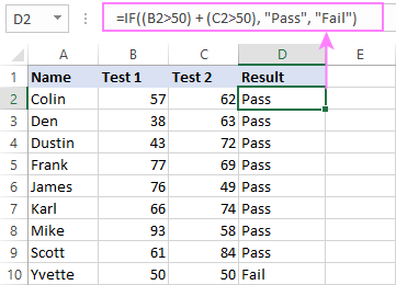
In my Excel 365, a normal formula works just fine (as you can see in the screenshots above). In Excel 2019 and lower, remember to make it an array formula by using the Ctrl + Shift + Enter shortcut.
To evaluate multiple conditions with the OR logic, the formula is:
=IF((B2>50) + (C2>50), "Pass", "Fail")
Using IF together with other functions
This section explains how to use IF in combination with other Excel functions and what benefits this gives to you.
Example 1. If #N/A error in VLOOKUP
When VLOOKUP or other lookup function cannot find something, it returns a #N/A error. To make your tables look nicer, you can return zero, blank, or specific text if #N/A. For this, use this generic formula:
For example:
If #N/A return 0:
If the lookup value in E1 is not found, the formula returns zero.
=IF(ISNA(VLOOKUP(E1, A2:B10, 2,FALSE )), 0, VLOOKUP(E1, A2:B10, 2, FALSE))
If #N/A return blank:
If the lookup value is not found, the formula returns nothing (an empty string).
=IF(ISNA(VLOOKUP(E1, A2:B10, 2,FALSE )), "", VLOOKUP(E1, A2:B10, 2, FALSE))
If #N/A return certain text:
If the lookup value is not found, the formula returns specific text.
=IF(ISNA(VLOOKUP(E1, A2:B10, 2,FALSE )), "Not found", VLOOKUP(E1, A2:B10, 2, FALSE))

For more formula examples, please see VLOOKUP with IF statement in Excel.
Example 2. IF with SUM, AVERAGE, MIN and MAX functions
To sum cell values based on certain criteria, Excel provides the SUMIF and SUMIFS functions.
In some situations, your business logic may require including the SUM function in the logical test of IF. For example, to return different text labels depending on the sum of the values in B2 and C2, the formula is:
=IF(SUM(B2:C2)>130, "Good", IF(SUM(B2:C2)>110, "Satisfactory", "Poor"))
If the sum is greater than 130, the result is "good"; if greater than 110 – "satisfactory', if 110 or lower – "poor".
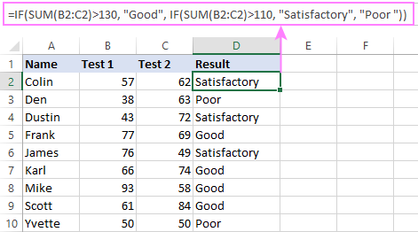
In a similar fashion, you can embed the AVERAGE function in the logical test of IF and return different labels based on the average score:
=IF(AVERAGE(B2:C2)>65, "Good", IF(AVERAGE(B2:C2)>55, "Satisfactory", "Poor"))
Assuming the total score is in column D, you can identify the highest and lowest values with the help of the MAX and MIN functions:
=IF(D2=MAX($D$2:$D$10), "Best result", "")
=IF(D2=MAX($D$2:$D$10), "Best result", "")
To have both labels in one column, nest the above functions one into another:
=IF(D2=MAX($D$2:$D$10), "Best result", IF(D2=MIN($D$2:$D$10), "Worst result", ""))

Likewise, you can use IF together with your custom functions. For example, you can combine it with GetCellColor or GetCellFontColor to return different results based on a cell color.
In addition, Excel provides a number of functions to calculate data based on conditions. For detailed formula examples, please check out the following tutorials:
Example 3. IF with ISNUMBER, ISTEXT and ISBLANK
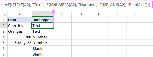
To identify text, numbers and blank cells, Microsoft Excel provides special functions such as ISTEXT, ISNUMBER and ISBLANK. By placing them in the logical tests of three nested IF statements, you can identify all different data types in one go:
=IF(ISTEXT(A2), "Text", IF(ISNUMBER(A2), "Number", IF(ISBLANK(A2), "Blank", "")))
Example 4. IF and CONCATENATE
To output the result of IF and some text into one cell, use the CONCATENATE or CONCAT (in Excel 2016 - 365) and IF functions together. For example:
=CONCATENATE("You performed ", IF(B1>100,"fantastic!", IF(B1>50, "well", "poor")))
=CONCAT("You performed ", IF(B1>100,"fantastic!", IF(B1>50, "well", "poor")))
Looking at the screenshot below, you'll hardly need any explanation of what the formula does:

IF ISERROR / ISNA formula in Excel
The modern versions of Excel have special functions to trap errors and replace them with another calculation or predefined value - IFERROR (in Excel 2007 and later) and IFNA (in Excel 2013 and later). In earlier Excel versions, you can use the IF ISERROR and IF ISNA combinations instead.
The difference is that IFERROR and ISERROR handle all possible Excel errors, including #VALUE!, #N/A, #NAME?, #REF!, #NUM!, #DIV/0!, and #NULL!. While IFNA and ISNA specialize solely in #N/A errors.
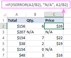
For example, to replace the "divide by zero" error (#DIV/0!) with your custom text, you can use the following formula:
=IF(ISERROR(A2/B2), "N/A", A2/B2)
And that's all I have to say about using the IF function in Excel. I thank you for reading and hope to see you on our blog next week!
Practice workbook for download
Excel IF multiple criteria - examples (.xlsx file)
 by
by
4506 comments
Hi trying to build the following formula:
If Cell G3 = 1 and Cell I3 = 36 Return "-2"
If Cell G3 = 1 and Cell I3 = 37 Return "-3"
If Cell G3 = 1 and Cell I3 = 38 Return "-4"
The formula I have written is:
=IF(AND(G3="1"(I3>37,"-4",IF(I3=37,"-3",IF(I3=36,"-2","0")))))
This doesn't appear to work. Could you help?
Hi Russ,
Try the following syntax:
=IF(AND(G3=1,I3>37),-4, IF(AND(G3=1,I3=37),-3, IF(AND(G3=1,I3=36),-2,0)))
Please note that in Excel formulas, you should not enclose numbers in double quotes unless you want them to be treated as text values.
Hi, I'm trying to build a formula with 3 logic tests as follows:
If cell E4 is blank then = blank
If cell G4 plus 29 days is < today’s date then = Compliant
If cell G4 plus 28 days is < today’s date then if true = Review required if not Overdue
Below is what I have in Excel
=IF(ISBLANK(E4),"", IF((G17+29)<TODAY(),"Compliant",IF((G4+28)<TODAY(),"Overdue","Review required"))
Everything appears to work except for IF((G17+29)<TODAY(),"Compliant"
What is wrong with my formula?
Hi Claire,
That's probably because in your formula it's IF((G17+29)<TODAY() while the condition reads "cell G4 plus 29 days". Please check this.
Hi,
I need your help with a simple formula but it`s giving me a hard time. I need the result to be
if(b=0,"100", if(f=0,0), if not f/b
I do not seem to make the formula work. Would you please help?
Guddu,
A1 being previous sales, A2 being current sales.
=IF(A1>A2,A1,A2)
i want to create a marks card, as like class 12th marks card in india , so plz which formula i use in it give me all..
If I compare two year sales and amount of previous one is greater than present month then the result will show the greater one.
Please help
awesome way too helpful .. thanks alot
Ok. Here is my issue. I am trying to reference another sheet(Sheet1) and run 2 logical tests and return the value of the corresponding B column of any that match the tests. This is what I used
=IFERROR(INDEX(Sheet1!$B$2:$B$5000,SMALL(IF(AND(""=Sheet1!$AX$2:$AX$5000,"YES"=Sheet1!$CV$2:$CV$5000),ROW(Sheet1!$AX$2:$AX$5000:Sheet1!$CV$2:$CV$5000)-ROW($A$2)+1),ROW(1:1))),"")
When the logical if statements are done separately they seem to work but together they do not. this is a modified version of this formula
=IFERROR(INDEX(Sheet1!$B$2:$B$5000,SMALL(IF("NEW"=Sheet1!$O$2:$O$5000,ROW(Sheet1!$O$2:$O$5000)-ROW($A$2)+1),ROW(1:1))),"")
This formula is similar and works but I have not been able to get 2 logical tests to work together properly.
Anyone willing to give this one a shot that would be awesome.
I am trying to create a formula to reference a certain cell's text. What I want it to do is input a value based on what text is in a certain cell. For example, I want it to refer to cell E6 and if it is biannual, I want it to input 2. If it's annual, I want it to input 1, if it's monthly, I want it to input 12, and if it's quarterly, I want it to input 4. Can it do something like that?
Yes. That should be very simple to create. Multiple (If) statements will get that done.
Hi,
IF A1 is greater than A2 then value=B1, and if A1 is greater than A3 then value=b2 or B1.
I am calculation plan value for my forecasted date vs my data date. Kindly advise.
Thanks.
I need an IF formula for:
IF P20 equals 83-100, Highly Effective
IF P20 equals 66 – 82, Effective
IF P20 equals 53 – 65, Needs Improvement
IF P20 equals 0 - 52, Unsatisfactory
Hi Jackie,
You need a nested IF formula like this:
=IF(P20>=83, "Highly Effective", IF(P20>=66, "Effective", IF(P20>=53, "Needs Improvement", "Unsatisfactory")))
Looking for assistance with the following:
If the date in E2 is prior to today AND L2 is less then 0 then return CHECK if false then return OK
Hi Stacey,
Here you are:
=IF(AND(E2<TODAY(), L2<0), "CHECK", "OK")
IF A1= "any value" then A1= sum of B1,B2 or "zero"
Please advise. Thanks.
Hi Riyaz,
Here you go:
=IF(A1<>"", B1+B2, 0)
Thank you so much Svetlana Cheusheva
A1 = RECEIVED / CANCELLED / DECLINED (Dropdown)
If A1="CANCELLED" then A2, A3, A4... will show CANCELLED
If A1="DECLINED" then A2, A3, A4... will show DECLINED
but
If A1="RECEIVED" then A2, A3, A4... must be blank
Please advise. Thank you
HI BRENDA,
TRY THIS
=IF(A1="CANCELLED","CANCELLED","")&IF(A1="DECLINED","DECLINED","")&IF(A1="RECEIVED","","")
Hi Svetlana,
I am having a bit trouble with the IF function with ISNUMBER and FIND/SEARCH to match and substitute strings. However, I am not getting the desired outcome. Let say, Cell 1 has string "Kara", Cell 2 has "Karam".This is my formula =IF((ISNUMBER(FIND(A1,A2))),SUBSTITUTE(A1,A1,A2),A2). Now, it is substituting Cell 1 string with Cell 2. However, I want it to substitute on the basis of full name. For instance, if Cell 2 had "Kara & Jones", then it should substitute, not only if the same characters are found. Any comments or directions would be highly appreciated!thx
Guys,
If you have any suggestions regarding my problem, I would be grateful!
I want to make this formula works:
if cell B2=0 then Cell C2=0 if cell B is not equal 0 then use this formula (C2*25)+25) to calculate the result of cell C2
Here i am attaching two sheets, One interest rate. The other interest charged. I want to have a clear sheet when ever there is change in interest based on the balance rate to be charged monthly. I want to know what the formula to be used.
sheet 1
FROM TO INT RATE
31-03-2011 24-04-2011 8.25
25-04-2011 11-05-2011 8.50
12-05-2011 10-07-2011 9.25
11-07-2011 12-08-2011 9.50
13-08-2011 19-09-2012 10.00
20-09-2012 03-02-2013 9.75
sheet2
DATE DR CR BALANCE NO.OF DAYS
31-03-2011 45455604 45455604 30 24 5
30-04-2011 394156 45849760 1
01-05-2011 394156 45455604 11
12-05-2011 3000100 42455504 19
31-05-2011 425189 42880693 1
01-06-2011 425189 42455504 29
30-06-2011 401292 42856796 1
01-07-2011 401292 42455504 7
08-07-2011 921233 41534271 23
31-07-2011 413676 41947947 1
01-08-2011 413676 41534271 30
31-08-2011 425299 41959570 1
01-09-2011 425299 41534271 29
30-09-2011 418187 41952458 0
01-10-2011 418187 41534271 30
31-10-2011 432127 41966398 1
01-11-2011 432127 41534271 2
03-11-2011 432127 41966398 14
17-11-2011 432127 41534271 13
30-11-2011 420218 41954489 1
01-12-2011 420218 41534271 30
31-12-2011 432127 41966398 1
01-01-2012 41966398 23
24-01-2012 66112 42032510 7
31-01-2012 370511 42403021 29
29-02-2012 412703 42815724 2
02-03-2012 432127 42383597 29
31-03-2012 441109 42824706 30
actually interest charged is 394156 but according to my cal Outstanding 45455604 * 24 days *8.25%/365 + 45455604*5 days *8.50/365 should be my interest
What is the formula used by combing sheet 1 and sheet2 to calculate the interest
Using Google Sheets.
I have a formula that is using validated data to display a value in a field:
=IF(H3="0X0", "$0.00", IF(H3="12 x 2", "$120.00", IF(H3="15 x 3", "$220.00", IF(H3="19 x 4", "$380.00", IF(H3="10 x 7", "$350.00")))))
This works perfectly, however, I cannot get total of the values returned. I am using the following formula: =Sum(I3,G3,E3,C3)
Don't worry I figured it out: remove the '$' from the formula and use =Sum(I3+G3+E3+C3)
Using Google Sheets.
I have a formula that is using validated data to display a value in a field:
=IF(H3="0X0", "$0.00", IF(H3="12 x 2", "$120.00", IF(H3="15 x 3", "$220.00", IF(H3="19 x 4", "$380.00", IF(H3="10 x 7", "$350.00")))))
This works perfectly, however, I cannot get total of the values returned. I am using the following formula: =Sum(I3,G3,E3,C3)
I have three worksheets that contain about 50 customer names. How can I assign the salesman name (forth worksheet) to each customer? I would like to do something like: if sheet1 list customer xxx, yyy and zz,their salesmen is A.
Thanks for the advise
HOW TO FIND EARLIEAST DATE CELL CONTAINS TEXT AND D DATE . 28 29-Nov-15 02-Dec-15 09-Dec-15 55 06-Dec-15 09-Dec-15 16-Dec-15
NO THANKS AND I WILL FIND THE ANSWER
HOW TO DO THIS QUESTION
CALCULATE THE CHARGE VALUE BY USING IF FUNCTION
Name units charge
raja 250 condition
kumar 150 0 to 200 - 1UNIT - Rs 6
sasi 800 200 to 500 - 1UNIT - Rs 9
mala 469 >500 - 1UNIT - Rs 12
raciga 640
uthayan 68
susila 342
CALCULATE THE CHARGE VALUE BY USING IF FUNCTION
Name units CHARGE
raja 250
kumar 150
sasi 800
mala 469
raciga 640
uthay 68
susila 342
Thanks, found this really useful! :)
Hi Svetlana, I really love your site, it has helped me multiple times.
I'm currently trying to figure out a way to efficiently write a nested if statement that doesn't involve manually writing it, as I will have 52 nested ifs when finished. I was trying to concatenate the pieces of my formula, but I'm having no luck. Do you have any other ideas? Ultimately what I'm trying to do is have Excel look in one column for a value >0 and if it detects it, show a value from an adjacent cell....then I want to average those numbers.
I need a formula that does the following:
IF the value in cell B1 is BLANK, then return "BLANK"
IF the value in cell B1 is TEXT, then return "Available"
IF the value in cell B1&C1 is TEXT, then return "Filled"
I need help with a formula for conditional formatting.
IF cell D12 is blank and the date in cell C12 is within 14 days of today's date, then the text is formatted red.
Hi Carrie,
Does "within 14 days of today's date" mean 14 days in the past or in the future?
If the target date in C12 is less than 14 days from today.
So, target date is 11/15/15 it would be highlighted because it is due within 14 days.
Hi Carrie,
Select the cells (or rows) you want to format red beginning with row 12 and create a conditional formatting rule will the following formulas:
=AND($D12="", $C12>TODAY(), $C12-TODAY()<14)
Svetlana, it worked perfectly! Thank you for your assitance!
Hi Svetlana
I need a formula which shows the result of two different cell for example
the input from the two cell
1) 97130327 or 811045
2) negative(-) or positive(+)
result in cell
A) If first two character of the first cell is "97" & figure in second cell is positive then result will be "27" & if the second cell is negative then the result will be "37"
B) If first two character of the first cell is "81" & figure in second cell is positive then result will be "40" & if the second cell is negative then the result will be "50"
RESULT 1 CELL 2 CELL
37 97130127 (1000.00)
27 97130127 1000.00
50 811045 (1000.00)
40 811045 1000.00
Hello,
I am needing to integrate a formula into excel to calculate a tiered pricing schedule. The formula needs to assess if the cell value falls into one of 36 different ranges and than multiplies the cell value by a multiplier specific to that range. For example if the cell falls into the range of >5 and 15 and <=30 multiply by 9.33 and so on.
Schedule Example
Range Markup
1 5.01 to 15.00 9.37
2 15.01 to 30.00 9.33
3 30.01 to 55.00 9.30
............ ...
34 9505.01 to 9999.99 4.30
Example Correction: For example if the cell falls into the range of > 15 and <=30 multiply by 9.33 and so on.
Hi Svetlana,
I want to use a formula to match many specific, unique numbers to unique descriptions for two columns. Example is a 7 or 8 digit number (40307014) = specific description. I want to just be able to type in the unique number and have the description pop up automatically that matches the specific number. Do you have any formulas pre-written for this or advice on how to do this?
Thank you!
Hello Excel GURU,
Could you suggest a unique formula for below issue where the last column should automatically refill from formula. 10 till column 6 (for GOLD), 13 till column 12 (for DIAMOND), 25 till column 18 (for SILVER) and so on as I have big list for same criteria.waiting for your helpful response. Thanks in advance!
Serial No. GOLD 10
712755 $10.95
713296 $10.10
717453 $9.99
713812 $9.95
716291 $10.10
Serial No. DIAMOND 13
712755 $9.10
713296 $8.85
717453 $8.99
713812 $9.90
716291 $7.99
Serial No. SILVER 25
712755 $8.00
713296 $7.99
717453 $6.99
713812 $7.75
716291 $7.50
Hello,
I have stages called, 1-2,1-3,1-4 and so on and I need to called these all as Stage 1. Kindly help me how and which formula I can use for this.
Thanks,
Ashish
Hello. I have a cell that I input a simple IF statement into. For example, the formula was "=IF(C2<C3,"PASS","FAIL"). C2 and C3 are both elevations that were calculated with a simple formula also. An example of a formula for C2 or C3 might look like "=380.10 - (.02*10)" where 380.10 is a previous elevation and .02 is a slope in ft/ft and 10' is a width in feet. If the first formula returns a "pass" value, can excel tell me, and show me, which slope value made the statement true? The slope could be one of several different numbers such as .01,.02,.03,.04, and so on.
How do you nest formula across 3 or more columns to pull data from one column if another is blank? letters only no numbers or grades. I want to pull from Col 1, if not Col 2 then Col 3 when blank
Col 1 Col 2 Col 3 RESULT
1. aaa A aaa
2. bbb B bbb
3. - - - N/A
4. AA AA
5. C C
6. B+ B- B+
Thank You,
Bob
I HAVE THE BELOW DATA
IF DATE RANGE IS >361 show p1
if date range is 241 show p2
121 show p3
61 show p4
<=60 show p5.
Can u help me with the formula which can auto populate the data based on this 5 date criteria.
I have a date range of data based of which i want the data to populate.
the range is >361 it should show P1
241 show P2
Could you please help me to put the formula for the following conditions:
95-100 A
90-94 A-
87-89 B+
84-86 B
80-83 B-
74-79 C+
66-73 C
61-65 C-
56-60 D+
50-55 D
00-49 F
SUPER
hello!
I'm trying to create a formula wherein:
Cell value needs to check if it is Stop, Pending and Others.
Checks the Value in another cell it is pending or not then the condition in the table applies. wherein the cell value result will be the size.
Size Category Stop Pending& Others
X-Small <=1 <=1
Small <=3 <=2
Medium <=10 <=6
Large <=20 20 > 15
I'm trying to use a formula to return a value using multiple conditions as shown in this table:
FE Gross PVR
Units 1,450 1,500 1,550 1,600 1,650 1,700
220 32 33 34 37 39 40
210 31 32 33 36 38 39
200 30 31 32 35 37 38
190 26 27 29 32 33 34
180 25 26 28 31 32 33
170 24 25 27 30 31 32
Example: If Units are >189 and less than 1499 and less than 1550, then return the value of 27.
I would appreciate any assistance. Thank you!
for some reason the formulas post here show different what the one i write
=IF(A1>=37,10000,IF(A1>=28,1000),IF(A1>=19,100),IF(A1>=10,10),IF(A1>=1,1))
Hi!
You were almost there. You just have to close all IF's at the end of the formula, like this:
=IF(A1>=37,10000,IF(A1>=28,1000,IF(A1>=19,100,IF(A1>=10,10,IF(A1>=1,1)))))
i also use this
=IF(AND(A1>=1,A1=10,A1=19,A1=28,A1=37),10000,A1)
but it come back #VALUE
I tried all your exaples for an issu i have but non of them comes with the correct answer
i have a series o number for some score that need to be analyzed
12 16 21 33 45
i need to use a formula where is a number falls between a range of number to come back with another result this is my list
1-9 1
10-18 10
19-27 100
28-36 1000
37-45 10000
this is what I came up with
=IF(AND(A1>=1, A1=10, A1=19, A1=28, A1=37),10000,A1)))))
i also use this as a test
=IF(A1<=37,10000, IF(A1<=36,1000,IF(A1<=27,100, IF(A1<=18,10,IF(A1<=9,1)))))
but it only get th the first if statement
I am trying to write an IF statement formula for the following condition:
This is TEXT only, no numbers.
If Column F is blank, import the text value from Column K (same row)
If Column F is not blank, leave it as-is.
Hi,
My data reads:
Status Category
Successful Normal Minor.Production
Successful Normal Minor.Production
Successful Normal Minor.Production
Successful Standard-Minor
Successful Standard-Minor
Successful Normal Minor.Production
I want to compare both the columns for text and return a different text eg: "Successful Minor". I used this statement =IF(AND(C3 = "Successful", E3 = "Minor"), "Minor Successful", ) but this means the column B needs to specify minor. How do I do text search? Hope my question is clear. Appreciate your assistance.
Thank you kindly
Regards,
-V-
Hi .. I am trying to set a formula to calculate a hotel room rate based on the day of week. If Fri, Sat, Sun then $230 and if Mon-Thu $240. Person needs to enter arrival date 1/8/2016 .. then this reports back Fri (=c6 with the custom formatting of ddd)
Ex
Cell C6 has 1/8/2016, then C5 is set to =c6 (custom formatting of ddd). The formula I have is IF(C5="FRI","$230","$240").
Problem is C5 does not read FRI and is shows, but reads as =C6 and $240 is returned.
Any help in getting the formula to recognize day of week that is returned off a formula.
Thank you
I need help!
Conditions:
If sales are greater or equal to 10 then multiply the named cell RateA by Cost
If sales are greater or equal to 20 then multiply the named cell RateB by Cost
If sales are greater or equal to 30 then multiply the named cell RateC by Cost
Hello and please help.
Take Row A through L
If A1 equals K1 then L1 needs to move to B1
How to formulate this
=If(A1=K1;L1=B1) ?????
Hi Luke,
Here's the formula for B1:
=If(A1=K1, L1, "")
The formula will copy a value of L1 to B1 if A1=K1.
Sorry something went wrong ... below the Table again ...
I need a formula (If I guess) create a new Score from the NOT PASS (less than 50) an individually new PASS Score in another cell. I tried many things but failed ... I think it should be like ... The difference from PASS Score to NOT PASS Score plus some individually value added from the difference.
Ehm is ... Thank you all for help and understanding my bad English. I can explain it in German, but this is an english writing/reading forum. Smile
U1 U2 Part Read completed Write Point Score
79 87 10 10 10 10 10 100 50
78 99 6 7 8 6 5 57 55
78 95 5 5 8 6 5 50 58
76 77 5 3 8 8 5 12 16
79 89 6 3 8 4 8 23 35
62 19 6 2 5 5 5 19 26
71 14 5 4 8 L 5 53 45
73 49 4 3 8 6 7 32 31
34 9 5 5 8 5 5 27 23
77 87 5 7 8 5 5 38 29
71 17 5 2 5 4 8 9 18
Sorry ... I cant figure it out ... what happen to the table in my post. I formated in Courier ...
Hello ... I need a formula which counts the difference between the pass score >50 and the not pass score <50 and creates an individual pass score depending on the difference from the no pass score to the pass score.
Sorry my english ... I guess it will be an multiple IF and Formula ...
Thank you for advice and help
U1 U2 Part Read completed Write Point Sco
79 87 10 10 10 10 10 100 100 50
78 99 6 7 8 6 5 57 55
78 95 5 5 8 6 5 50 49 58
76 77 5 3 8 8 5 12 16 25
79 89 6 3 8 4 8 23 26 35
62 19 6 2 5 5 5 19 17 26
0 9
71 14 5 4 8 L 5 53 45 54
73 49 4 3 8 6 7 32 31 40
34 9 5 5 8 5 5 27 23 32
77 87 5 7 8 5 5 38 39 48
71 17 5 2 5 4 8 9 9 18